|
|
|
|
|
|
The Self-Capacitance of Toroidal Inductors.
|
1. Introduction. 2. Experimental method. |
3. Data reduction. 4. Relationship between self-C and N. |
|
A resonance method was used to determine the self-capacitances of a number of small toroidal inductors with single-layer windings. The data are interpreted on the basis that an inductor behaves as a short-circuited transmission line, with an additional lumped capacitance (the gap capacitance) in parallel with the terminals due to the toroidal structure. It is found that the self-capacitante tends towards a constant value which is greater than the gap capacitance as the number of turns (N) increases. This finite 'non-electrostatic' component of self-capacitance is consistent with the view that the propagation velocity is relatively close to the speed of light, i.e., the energy in transit is not concentrated within the high refractive-index medium provided by the core. Empirically, the self capacitance above the limiting value for large N is roughly proportional to 1/N². Data for different wire diameters can all be fitted to the same regression function, thereby excluding the hypothesis that self-capacitance is due to the capacitance between adjacent turns. |
|
1. Introduction: The self-capacitance of magnetically-cored coils with multi-layer windings is discussed in E C Snelling's masterwork on soft ferrites [12]. On the matter of coils with single-layer windings however, these being the focus of interest for the radio engineer, Snelling recommends the use of Medhurst's formula [Medhurst 1947]. The problem here is that Medhurst's data relate to solenoid coils with non-magnetic cores. It is also the case that Medhurst used what amounts to transmission-line theory to arrive at the long-coil limiting behaviour for his semi-empirical formula. It is commonly assumed that Medhurst's findings are consistent with the idea that self-capacitance in single-layer coils is due to capacitance between adjacent turns, whereas in reality, they show most decisively that it is not. Given that we need to consider the propagation of electromagnetic energy along the winding-wire in order to deduce the behaviour of un-cored solenoids; it follows that we will need to do the same for the case when a magnetic core is present. The core changes the electromagnetic environment, and so it is conceiveable that Medhurst's formula will not be applicable without modification. Furthermore, even if we can adapt Medhurst's results, there is a difficulty in that he provides only a method for estimating self-capacitance from coil geometry in the limit that the number of turns is large. One of the main points in using magnetic cores in RF applications is to obtain substantial inductance with the minimum length of winding wire; and in general, this implies a low number of turns. In view of the unsatisfactory situation described above, the following study was undertaken. A particular objective was to quantify the self-capacitance of the type of small toroidal coil typically used to make radio-frequency current transformers. A decision was made to adopt a fixed geometry; that of a bead of ½" (12.7mm) outside diameter, with a roughly constant gap between the ends of the winding. In that case, the only variables to be reconciled are the number of turns, the thickness of the wire, and the permeability of the core material. This imposed limitation, of course, implies that the findings may not be applicable to coils of other sizes; but the relationships extracted turn out to be particularly simple and amenable to theoretical analysis. |
|
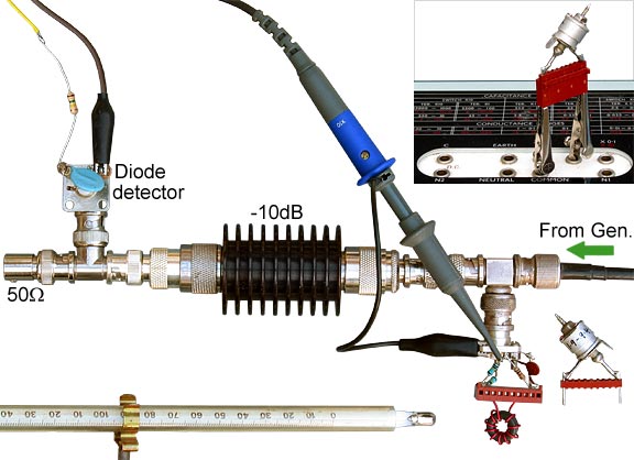
2. Experimental method: The method used for measuring the self-capacitance of the test coils is that of G W O Howe. It involves resonating the coil against a series of known capacitances, fitting the data to a regression line, and extrapolating to find the resonant frequency when C=0. The experimental setup for the present study is shown below. |
 |
 |
 |
 |
|
For measurements in the range 1.6 MHz to 30 MHz, the generator
was a Kenwood TS430s
radio transceiver adapted to be continuously tuneable in transmit
mode. It was terminated in a 50 Ω load consisting of a
-10 dB T-attenuator and a 50 Ω coaxial resistor. A diode
detector, connected to a T-piece between the attenuator and the
resistor, was used to monitor the transmitter output; the chosen
level for the experiment being about 10 W (22 V RMS at the test
jig). The drive voltage makes no difference to the resonant frequency,
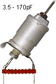
and is controlled merely to avoid overheating the load. A small number of measurements were made above 30 MHz using a signal generator with an output of about +3 dBm. In these cases, the oscilloscope response was feeble but still sufficient to determine the resonant frequency with reduced accuracy. The purpose of such measurements was to explore breakdown of the lumped-component model, and none were included in the least-squares analysis. The test jig is built onto the back of a BNC socket. The resonant circuit is excited via a 100 kΩ resistor, and the high-impedance (parallel resonant) condition is determined by sampling the voltage across the resonator using a potential divider. A ×10 probe (10 MΩ // 2 pF) connected to a 100 MHz oscilloscope was used tor the voltage measurement. A 3.3 pF nominal (3.1 pF actual) capacitor was connected across the probe connection points to swamp the probe capacitance; its purpose being to minimise the error in calculating the parasitic capacitance of the jig from measurements made with the probe disconnected. The jig is fitted with a socket, allowing the reference capacitor to be removed and measured on a laboratory bridge. The distance between the connecting pins is 1" (25.4mm), and unused pins and receptacles were removed in order to minimise strays. Capacitance measurements were made at a frequency of 107 radians/sec (1.5915 MHz) with a standard-deviation of measurement accuracy of somewhat better than 1% for large values and 0.05 pF for small values. For the majority of the measurements reported here, three variable reference capacitors were used, depending on the capacitance needed to achieve resonance. These were beehive trimmers; of nominal ranges 2 to 8 pF and 3.5 to 170 pF; and a small polyester-spaced receiver tuning capacitor for capacitances greater than 170 pF. The beehive trimmers were always mounted with the outer (rotatable) electrode connected to the ground terminal of the jig; and subsequently, to the common terminal of the measuring bridge. Handling was by means of forceps, holding the plastic part of the connector, to avoid disturbing the setting during transfer from the jig to the bridge. For each measurement, the capacitor was adjusted to peak the reading on the oscilloscope, and the generator frequency was then adjusted to see if the resonance could be located any more accurately. As the data acquisition progressed, a decision was made to speed-up the process by making a set of fixed plug-in reference capacitors. These were constructed using D-series 500 V silvered-mica capacitors with nominal tolerances of ±0.5 pF for values up to 47 pF and 1% for 56 pF and above. Capacitors were selected from batches of 5 of each value, the median sample being taken as best centred within the tolerance band as a check on the calibration of the measuring bridge. Finally, capacitors were mounted on plug-in headers, mostly singly, but in series an parallel combinations for some awkward values, and calibrated to within 0.6% (estimated standard-deviation) overall. The jig capacitance is due to the self-capacitances of the resistors and the strays across the jig itself. It was measured by disconnecting the scope probe and ground clip, fitting the BNC connector with a shorting-plug, soldering two short stiff wires in place of the device under test (DUT) and attaching them to the measuring bridge. A series of measurements were then made, with different fixed reference capacitors plugged into the capacitor socket, subtracting the known value of Cref from the total capacitance to obtain an estimate of the jig capacitance in each case. These estimates were then averaged, and the scatter used to determine the standard deviation, giving: C'jig = 0.72 ±0.05 pF this being the jig capacitance with the oscilloscope probe disconnected. Notice that the oscilloscope probe (nominally 2 pF input capacitance) lies in proximity to the various connectors during measurements. It was therefore assumed to add 3 ±1pF across the sampling point. If the resistors are considered to have parasitic capacitances of 0.3 pF each, it can be calculated that attaching the probe increases the jig capacitance by 0.011 ±0.002 pF. Hence the total jig capacitance is: Cjig = 0.73 ±0.05 pF The jig capacitance calculation is given in the spreadsheet file C_jig.ods. The reference capacitor and the connector, of course, also introduce parasitic inductance (about 50 nH). This however, is effectively in series with the inductance under test, and very small by comparison. Also, the conditions for most measurements were such that the reactance of the reference capacitor was large in comparison to the reactance of parasitic inductance. Hence it was not expected that correction for parasitic inductance would be needed. Such correction was included for some of the data adjustmants, but made no statistically-significant difference to the determined parameters and was eventually abandoned. |
|
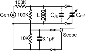
3. Data reduction: An inductor always has a self-resonant frequency (SRF), i.e., a frequency at which it will exhibit parallel resonance with no capacitor in parallel. Hence, the lumped-component model for an inductor operating at radio frequencies (neglecting losses), is an inductance in parallel with a parasitic capacitance, the latter being known as the 'self-capacitance' or (somewhat unrigourously) the 'distributed capacitance' of the coil. In fact, the concept of self-capacitance as a purely electrostatic energy-storage mechanism is invalid, the coil is best treated as a transmission line; but it has some utility for the purpose of circuit design, and it is therefore relevant to try to quantify it. In the lumped component model shown below, the inductor has a self-capacitance CL, Cjig is the parasitic capacitance of the measuring setup, and Cref is the variable experimental parameter. Hence, the total external capacitance contributing to the resonant frequency of the system is: |
|
C = Cjig + Cref In the event that the test coils all have reasonably high Q (which they do) the resonant frequency is given by: f0 = 1/{ 2π√[L(Cjig + Cref + CL)] } This can be rearranged to: |
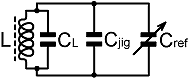 |
|
L (Cjig + Cref
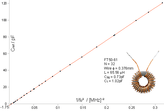
+ CL) = 1/(2πf0)² and hence: Cref = -(CL + Cjig) + [1/(4π²L)] (1/f0²) This is the equation of a straight line graph of the form y=a+bx, where: y=Cref , a=-(CL+Cjig) , b=1/(4π²L) , and x=1/f0² When an estimate of the jig capacitance is available (0.73 ±0.05 pF in this case), the self-capacitance of a coil (and, as a byproduct, the inductance) can be determined by taking a set of measurements of Cref vs 1/f0² and fitting them to a regression line. A weighted linear regression procedure [see Data Analysis] was used for this work because it allows different capacitance measurements to have different standard-deviations. It also allows anomalous measurements to be excluded from the fit, this being an important feature when the theoretical model is expected to break-down at some point. The regression line for one of the test coils is shown as an example below. The raw data are given in the open-document spreadsheet file: F61-32T.ods. |
|
In this case, the line crosses the y-axis at -1.75 pF. Allowing
for a jig capacitance of 0.73 ±0.05 pF, this gives the
coil self-capacitance (including the stray capacitance of the
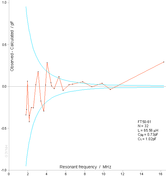
leads) as 1.02 ±0.05 pF. The regression procedure is convincing when illustrated as in the graph above, and appears to vindicate the lumped-component model. There is more information to be had however by examining the data in a manner that shows-up the experimental noise. To this end, a graph of the differences between the measured and calculated values of the reference capacitance (the fitting residuals) is shown plotted below. |
|
In addition to the data, the graph also shows the limits corresponding
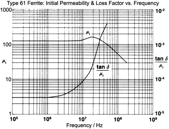
to one standard-deviation (1σ) of the error function: σCref = √[0.01² + (0.008Cref)² ] This function has been gerrymandered to bring the reduced χ² for the fit (the variance of an observation of unit weight) to unity. It represents a basic precision of capacitance measurement of 0.8%, with a 0.01 pF allowance for error in bridge nulling prior to a measurement. It does not necessarily represent a perfect choice, but no plausible adjustment will make a statistically significant alteration to the determined parameters. Bearing in mind that the most probable error in an observation is 1σ, the data show an extensive region which has the characteristic signature of normally-distributed random error. Hence the self-capacitance of the coil is well-defined over an interval of at least 3 octaves. At the HF extreme of the range however, the lumped-component model appears to break down; there being a single bad residual relating to the resonant frequency when no reference capacitor is plugged into the jig, i.e., when the coil is resonated against the jig capacitance alone. One possible cause of deviation above about 8 MHz is that the type 61 NiZn ferrite material used for the core is entering into a dispersion region (a region of changing initial permeability μi) as shown in the graph below. |
|
The problem of measuring the self-capacitance of windings on
fiercely dispersive (ultra-high permeability MnZn) ferrite materials
is examined by Yurshevich et al. [13].
Permeability dispersion is one of the reasons for the dearth
of good data on magnetically-cored coils. In the present work
however, the evidence is that the hump in permeability in the
8 to 30 MHz range of the manufacturer's graph is attenuated or
absent in the actual sample. The graph suggests an increase in
permeability of 28% between 8 and 18 MHz, and a fall thereafter.
Many of the datasets obtained span the region between 8 and 30
MHz, but all give good straight regression lines, with no statistically
significant curvature except at the extreme HF end. Prior to
the experiment, there was a plan to obtain an empirical expression
for the permeability profile and use it to correct the data,
but the exercise proved to be unnecessary. Permeability variation
simply cannot account for the pattern of deviation observed.
Later on, we will see that there is evidence of core dispersion
in some datasets, but it manifests itself as an anomalous AL value (a tilt in the regression line hidden
in the noise) when the dataset is truncated due to the 30 MHz
maximum frequency limit imposed by the generator.. For the true source of the HF deviation; is telling that it occurs in all of the datasets acquired by the author, regardless of whether or not the coil has a magnetic core. It is not associated with any particular measurement frequency, but it always occurs when the external resonating capacitance is comparable to or smaller than the extrapolated self-capacitance of the coil. One possible explanation is given by the Corum brothers and others [see refs on self-resonance page], who show that a helical conductor is a dispersive transmission line. The velocity factor for EM propagation is likely to change rapidly around the SRF, in which case the lumped-component model will cease to be valid in this region. It must also be noted however, that when the connected capacitance is small, the current through the coil can become non-uniform, and since inductance is associated with current, the effect might be attributed to a reduction in the effective inductance. From the foregoing, it should be clear that the assumption of constant self-capacitance and inductance is only valid at frequencies well below the SRF and cannot be used to predict the SRF. Self-capacitance is nevertheless a useful parameter for the purposes of circuit design, and it is well defined over an interval of several octaves. |
|
4. Relationship between CL and
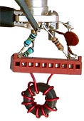
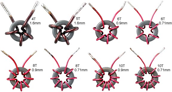
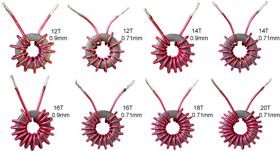
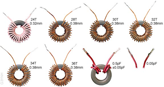
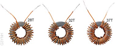
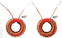
N: If we wish to design circuits on the basis of the impedance looking into the terminals of an inductor, at frequencies well below the SRF; it is useful to consider a toroidal coil as a solenoid with a lumped capacitance (the gap capacitance) connected across it. The gap capacitance is a true capacitance, due to the proximity of the emerging wires, and must be controlled if there is to be any meaningful comparison between different coils. An attempt to do so has been made for the set of coils shown below, and the extent to which the exercise was succesful will be discussed shortly. An attempt was also made to estimate the gap capacitance, by wrapping two pieces of wire around the core and gapping them about the same as for the coils, as shown in the penultimate photograph. |
|
The coils shown above were all wound on a single example of an
Amidon FT50-61 bead. (nominal μi=125).
The reason for using the same core for every self-capacitance
determination in this set is that all of the inductances determined
from the fitting parameters should return the same AL
(L/N²) value. As mentioned earlier, the core material is
dispersive, and the extraction of an anomalous inductance from
the fitting procedure is indicative of skewed data. The core
used had an AL value of about 64 nH/turn²
over the 2 MHz to 30 MHz range when averaged over the whole interval.
This is close to the manufacturer's nominal value of 69 nH/turn²,
showing that the core was not cracked or otherwise defective.
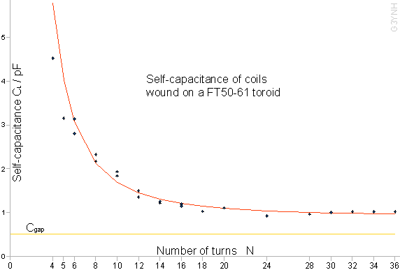
For each coil in turn, a set of Cref vs. f0 data was acquired and subjected to a regression analysis as described in the previous section. Note that for turns numbering 6, 8, 10, 12, 14 and 16, the measurements were duplicated with different wire diameters. In this way it was established that there was no statistically-significant wire-diameter effect. The individual spreadsheets were then pasted, as separate sheets, into a single spreadsheet file (f61_Cself.ods), so that the extracted parameters could be subjected to a meta-analysis. Note that this final large file pushed the software used (Open Office 2.3) to the limit of its stability. Frequent program crashes occured during the final adjustment of the error functions; but mathematical integrity, as far as the author is aware, was unaffected. There appears to be an issue related to the large number of interlinked variables, and those wishing to experiment further with the data adjustment are advised to save their work often. The initial meta-analysis, without preconceptions regarding what would be found, was simply that of plotting a graph of self-capacitance CL vs. the number of turns N. From this, it was immediately obvious that the resulting curve was an exponential decay function. Hence the self-capacitances were fitted to a regression function of the form: CL = C∞ + C1/Np Where the power p to which 1/N is raised is an input parameter. By measuring the capacitance of a mock-up of the coil end-gap, as shown in a photograph above, the gap capacitance was estimated to be about 0.5 pF (including lead capacitance) for most of the coils. A pessimistic estimate for the standard-deviation of this figure can be had by noting that we can have near-perfect confidence that the true value lies between 0 and 1 pF. Hence, ignoring the skew due to the zero boundary, if we take 0.5 pF to be the 3σ confidence interval, then σCgap=0.17 pF. Hence, if the data scatter is primarily due to uncertainty in the gap capacitance, we need to get the σCgap component of σCL to be 0.17 pF or less for a reduced χ² of 1. In fact, we can do rather better than that by identifying the data for N=4 and 5 as anomalous (for reasons to be given shortly) and setting p=2. χ²/ν was brought to unity by using the error function: σCL = √(σ1² + 0.11²) [pF] where σ1 is the precision of the CL+Cjig value obtained from the first regression analysis. Hence we know that σCgap is better than or equal to 0.11 pF, which is realistic. The regression curve is shown below with the data superimposed. |
|
The data for N=4 and N=5 were excluded from the fit for two reasons.
Firstly, from the photographs above, it can be seen that these
two coils will have less gap capcitance than the others. Secondly,
the fits for both coils returned anomalously high AL
values. The problem here is that as the SRF moves to higher frequency,
the maximum measurement frequency of 30MHz necessitates extrapolation
to the self-capacitance from further and further away. The effect
of any slight variation of AL with frequency
will be amplified in this way. When the inductance returned from
the fit is higher than the true value, the self capacitance will
be lower than the true value. Hence we can account for the deviation. The empirical relationship obtained from the analysis is:
If the gap capacitance is about 0.5 pF, it appears that the non-electrostatic component of the self-capacitance settles to about 0.40 ±0.11 pF as the number of turns becomes very large. |
| >>> Notes for further work: |
|
Capacitance predicted by medhurst's formula: Average OD for coil wound with 0.376 mm wire. 5.3 mm Average dia. 5.1 mm Core OD=12.7, ID=7.1, Mean=9.9. Average circ.=31.1. Solenoid length=28 D/ 4ε0 Medhurst's formula in SI units:
CL = 0.3157 ( 1 + 0.12915 + 0.18596) CL = 0.3836 pF Spreadsheet: medhurst.ods . |
 |
FT50-67 core. Wire diam: 0.376mm Data: F67_CL.ods .
|
 |
T50-2 core Wire diam: 0.376mm Data: T50-2_CL.ods .
|
|
>>>>> Notes: >>> effect of dispersion on AL
. |
References and further reading
|
[12] Sort Ferrites:
Properties and Applications. E C Snelling. 2nd ed. Butterworth.
1988. ISBN 0-408-02760-6. Winding self-capacitance. p330-335. [13] Measurement of Self-Capacitance for windings on High-Permeability Ferrite Cores. V Yurshevich, S Lomov and J Jankovskis. Measurement Science Review, Vol 1, No. 1, 2001. p219-222. Available online: www.measurement.sk/Papers3/Yur.pdf . (Accessed 5th Jan. 2016) See also: |
© D W Knight 2008, 2015, 2016
David Knight asserts the right to be recognised as the author of this work.
|
|
|
|
|
|