| |
|
|
|
|
6.2 Current Transformers: Part 2.
10. Low-frequency performance:
The effective secondary parallel reactance of a current transformer in the low-frequency region of its passband is dominated by the inductance of the secondary winding. Hence, for the purpose of calculating the low-frequency response, the model can be simplified as shown below.
Here the capacitance has been ignored, and the inductance Li should be taken to be about 1 or 2% less than the measured inductance of the secondary coil. The relationship between primary current and secondary voltage (neglecting losses) given earlier as equation (4.1) is now reduced to:
| Vi = I (Ri // jXLi) / N |
The obvious implication is that there will be significant phase and amplitude errors in the output unless XLi >> Ri. In fact, the lower -3dB bandwidth limit occurs when XLi = Ri, with an attendant phase error of +45°.
Phase and magnitude errors in the current sampling network of a bridge will compromise the accuracy of the balance condition. We will see in later sections however, that compensation can be achieved by modifying the voltage sampling network so that its output has the same frequency response as that of the current sampling network. Such compensation however, does not correct for the low-frequency reduction in output voltage, and this has implications with regard to the sensitivity of bridges, and the accuracy of current-measuring instruments. It is therefore principally the desire for a flat amplitude response that dictates the minimum value of inductance that can be tolerated, and we can understand this issue by considering the simple RF ammeter circuit shown below:
Here the detector is sensitive only to the magnitude of the output voltage, and the reading on the meter (assuming a scale calibrated to allow for diode forward voltage drop) is given by:
Vmeas = (√2) |Vi|
where:
|Vi| = |I| |(jXLi // Ri)| / N
i.e.,
| Vmeas = (√2) |I| |(jXLi // Ri)| / N |
The measured output (i.e., the sensitivity) is therefore always proportional to the magnitude of the secondary load impedance, which (neglecting losses and the detector input resistance) consists of the secondary winding reactance in parallel with the load resistance.
The effect of placing an inductance in parallel with an impedance [discussed in Impedance Matching, section 5-7] is to move the resultant impedance anti-clockwise around a circle of constant conductance as the inductive reactance decreases. The reactance XLi=2πfLi, of course, decreases as the frequency decreases, and the constant conductance Gi is equal to 1/Ri. We can therefore visualise the process using the Z-plane diagram below:
Where Zi = (jXLi // Ri)
An expression for the magnitude of an impedance in its parallel form was given in [AC Theory, Section 18, eqation 18.2]. Using the present notation it becomes:
|Zi| = | Ri XLi / √( Ri² + XLi² ) |
At high frequencies, XLi becomes very large and its contribution to Zi becomes correspondingly small. In this capacitance-free model therefore, the magnitude of Zi can be considered to be equal to Ri at high frequencies, i.e., as XLi→∞, |Zi|→Ri. Consequently, since the measured voltage for a given input current is proportional to |Zi|, we can define a dimensionless amplitude-response function for the system as:
| ηLF = |Zi| / Ri = |XLi| / √ ( Ri² + XLi² ) |
(η is "eta", this time un-bold because the quantity it represents is scalar). The reason for deriving this expression, is that we can use it to obtain the minimum amount of inductance required in order to keep the drop in meter sensitivity within acceptable limits at the lowest frequency of operation. All we need to do is rearrange it until we have XLi expressed in terms of Ri and ηLF, as follows:
ηLF² = XLi² / ( Ri² + XLi² )
ηLF² ( Ri² + XLi² ) = XLi²
XLi² - ηLF² XLi² = ηLF² Ri²
XLi² (1 - ηLF²) = ηLF² Ri²
XLi² = Ri² ηLF² / (1 - ηLF²)
Now taking the square root to obtain XLi, we note that we only want the positive result (i.e., the magnitude of XLi), and so:
|XLi| = Ri ηLF / √(1 - ηLF²)
but since XLi is an inductive reactance, we know it will be positive and so we can dispense with the magnitude symbol in this instance (but not in general) to obtain:
| XLi = Ri ηLF / √(1 - ηLF²) |
The results for some possible design values for ηLF are tabulated below:
Table 10.1. Current transformer, low-frequency desensitisation and phase error.
|
=100(1-ηLF) |
=-20Log(ηfLF) |
=|Zi|/Ri |
=RiηLF/√(1-ηLF²) |
=Arcan(Ri/Xi) |
fmin=1.6MHz, Ri=50Ω |
|
|
|
|
|
|
|
|
|
|
|
|
|
|
|
|
|
|
|
|
|
|
|
|
|
|
|
|
|
|
|
|
|
|
|
|
|
|
|
|
|
|
The figure XLi ≥ 7Ri for 1% max. error is corroborated by ref [The ARRL Antenna Book, 19th edition, ARRL publ, 2000.
ISBN: 0-87259-804-7. Bridge types p27.4].
The data in the table tell us that if we want a current reading at the lowest frequency of operation (fmin) to be within 1% of a high-end reading of the same current, then XLi must be at least 7 times larger than Ri at the lowest frequency. If we want agreement within 5%, then XLi must be at least 3 times larger than Ri, and so on. The more stringent design requirements at the top of the table are appropriate for direct-reading RF ammeters, where scale accuracy is important; but for the design of RF bridges, where we are often in a position to turn up the generator level if the bridge sensitivity starts to fall, a reduction in sensitivity of 3dB, or even 6dB, may be perfectly acceptable.
Also shown in the table are the phase errors associated with the various design criteria. Notice that even when the amplitude is controlled to within 1%, the phase error at the minimum frequency is 8°. Underhill & Lewis [43] recommend that the maximum acceptable error for an impedance matching system should be ±7° (1.2:1 SWR), and so a large secondary inductance, notwithstanding the propagation-delay issue, is not a way of avoiding the need for phase compensation when designing bridges. We might, of course, decide to use a low value of load resistance and a large inductance; but that implies a low output voltage (i.e., insensitivity), which is fine when monitoring a transmitter producing kilowatts, but not so good when trying to tune an antenna using a few watts.
For those interested in designing accurate RF ammeters, note that using a large secondary inductance is neither the only, nor necessarily the best, way of obtaining a flat frequency response. By the inclusion of a capacitor, the secondary loading network can be modified to produce an output that is flat within 1% over the 1.6 to 30 MHz range (or greater) using an inductance of around 10 μH. This configuration, which does not appear to have been reported elsewhere, is referred to in these documents as the Maximally-Flat Current Transformer [see article of that name].
Ref:
[43] "Automatic Tuning of Antennae". M J Underhill [G3LHZ] and P A Lewis.
SERT Journal, Vol 8, Sept 1974, p183-184.
Gives criteria for achieving 1.2:1 SWR, i.e., 45 ≤ R ≤ 56Ω, 17.5 ≤ G ≤ 22.5 mS, -7° ≤ φ ≤ +7°.
11. LF phase-error demonstration.
A simple technique for demonstrating current-transformer low-frequency phase-error is illustrated below. It uses a method that works well at low frequencies (1.6 - 3 MHz) but can give misleading results at higher frequencies unless it can be shown that the oscilloscope Y-amplifiers have identical propagation delay and that the delay does not vary with the settings of the gain controls. In this case a waveform with the same phase as the primary current is obtained by measuring the voltage across a 50 Ω load resistor that terminates the generator. When this is compared with the voltage appearing across a 50 Ω resistor terminating the secondary winding, a phase difference is seen on the oscilloscope screen. By adjusting the Y-amplifier gain and shift controls, both waveforms can be made to have exactly the same height and be equally displaced about the central horizontal scale on the graticule. The phase difference between the two waves is then:
|
Δφ = |
Horizontal length of one cycle |
× 360° |
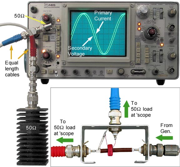
In the example above, the current transformer primary is a stub of URM108 (PTFE-Silver, 50Ω) cable, and the secondary is 61 turns of 36swg wire (0.225mm diameter including insulation) on an Amidon T50-2 (red) core. The published AL (inductance factor) for this core is 4.9nH/turns², giving a nominal secondary inductance (ALN²) of 18.2μH (± about 20%), but the measured inductance at 1.5915MHz (107 radians/sec) was 19.9±0.5μH. The phase-difference measurement was made at 1.6MHz, at which frequency the reactance of the coil (2πfL) is +200±5Ω. The situation shown on the oscilloscope screen is therefore XLi=4Ri.
The expected phase angle is:
Arctan(50/200±5) = 14.04±0.34°
Using the horizontal shift, timebase, and trigger level controls, the oscilloscope display was manipulated so that one cycle of the waveform was 10cm long. The distance between the zero-crossings of the two waves was then found to be 0.4 ±0.05cm. The measured phase difference is therefore:
360 × 0.4 / 10 = 14.40 ±1.8°
Which agrees with the calculated value.
On a practical point, notice that oscilloscope probes were not used, and that the signals were taken along 50Ω cables of equal-length and identical dielectric (for equal time-delay) and terminated at BNC T-pieces on the oscilloscope front panel. The problem with probes is that there will be capacitive coupling between them, and this gives rise to phase errors. The large transmitter terminator is shown hanging down from the front-panel; but a length of cable after the T-piece, so that the load can be placed more conveniently, is of no electrical consequence. The generator was a Kenwood TS430S radio transceiver with plug 10 removed from the RF module to give 1.6 to 30MHz transmitter coverage. The output level during the measurement was about 16Vp-p (5.7V RMS, 0.64W in 50Ω). No attenuator was used between the main transmitter line and the oscilloscope because it is important that both sampling points have the same input impedance (so that both cables are equally mismatched). For the instrument shown, both Y-amplifier inputs are 1MΩ // 20pF, which is typical.
12. Transformer core selection.
Having examined the basic design considerations for current transformers, we now turn our attention to the problem of choosing transformer cores from manufacturer's data. Here it will be assumed that we are primarily interested in designing current transformers for bridges, and a maximum low-frequency desensitisation of 3dB is acceptable; in which case the minimum secondary reactance must be no less than the load resistance. If the minimum frequency of operation is (say) 1.8MHz, and we intend to follow the normal practice of terminating the transformer with a resistor of about 50Ω, then the minimum secondary inductance Li=XLi/2πf=4.42μH. With this figure in mind, we may trawl the catalogues looking for cores that will fit reasonably tightly over a stub of coaxial cable, and which have AL (inductance / turns²) values that permit us to obtain a transformer ratio appropriate for our purpose.
Amidon supplies Micrometals and Fair-rite cores in small quantities (see also: links page for other sources). Hence, although suitable cores are available from various manufacturers, the use of Amidon products is convenient for private experimenters. Using the Amidon catalogue [38], and supplementary data from the Micrometals and Fair-rite websites, it transpires that the choice of core is remarkably limited once the frequency range and the hole diameter have been specified.
Ref: [38] Amidon Associates Inc. (Technical data book) Jan 2000.
Technical data for iron powder and ferrite cores, including AL values, frequency ranges, wire packing tables, Q curves, etc. Maximum flux density calculations and recommendations: p1-35. Information is also available online from: www.amidoncorp.com .
The point is that we need the core to be a tight fit on the cable in order to minimise leakage inductance and magnetic path-length; and so once a cable diameter has been chosen, the core hole diameter is the next size up that allows room for the secondary winding. The choice of core material is then that which gives sufficient secondary inductance with the required number of turns. The relevant information is summarised below:
Table 16.3. 50Ω PTFE Coaxial Cable data.
|
|
/ mm |
|
|
/ KV |
C0 / pF/m** |
factor |
| UR M72 |
|
|
|
|
|
|
| UR M102 |
|
|
|
|
|
|
| UR M107 |
|
|
|
|
|
|
| UR M108 |
|
|
|
|
|
|
| UR M109 |
|
|
|
|
|
|
| UR M110 |
|
|
|
|
|
|
| RG-142 |
|
|
|
|
|
|
| RG-303 |
|
|
|
|
|
|
| RG-316 |
|
|
|
|
|
|
| RG-393 |
|
|
|
|
|
|
| RG-400 |
|
|
|
|
|
|
Sources:
Uniradio Metric series data from: BICC Cableselector E15. PTFE Coaxial Cables. July 1979.
American Radio Guide series data taken from: The ARRL Antenna Book, 19th edition, ARRL publ, 2000. ISBN: 0-87259-804-7. Coaxial cable data p24-19.
* Coating materials vary / options exist - check manufacturer's data. NEVER use PVC in RF applications or where high temperatures may occur.
FEP = Fluorinated Ethylene Polypropylene. εr' = 2.1 (non-polar).
** Capacitance per unit length may vary depending on manufacturer. Inductance per unit length: L0 = 50²C0 .
Table 16.4. Toroidal Core Dimensions:
|
|
D /mm |
d /mm |
h /mm |
le / cm |
Ae / mm² |
/ mm |
|
|
|
|
|
|
|
|
|
|
|
|
|
|
|
|
|
|
|
|
|
|
|
|
|
|
|
|
|
|
|
|
|
|
|
|
|
|
|
|
|
|
|
|
|
|
|
|
|
|
|
|
|
|
|
|
|
|
|
|
|
|
|
|
|
|
|
|
|
|
|
|
|
|
|
|
|
|
|
|
|
|
|
|
|
|
|
|
|
|
|
|
|
|
|
|
|
|
|
|
|
|
|
Table 16.5. Maximum number of turns in single-layer winding:
|
|
/ mm |
(3.05 ID) |
(3.83 ID) |
(5.21ID) |
(5.82 ID) |
(7.62 ID) |
(9.40 ID) |
(12.6 ID) |
|
|
|
|
|
|
|
|
|
|
|
|
|
|
|
|
|
|
|
|
|
|
|
|
|
|
|
|
|
|
|
|
|
|
|
|
|
|
|
|
|
|
|
|
|
|
|
|
|
|
|
|
|
|
|
|
|
|
|
|
|
|
|
|
|
|
|
|
|
|
|
|
|
|
|
|
|
|
|
|
|
|
|
|
|
|
|
|
|
|
|
|
|
|
|
|
|
|
|
|
|
|
|
|
|
|
|
|
|
|
|
|
|
|
|
|
|
|
|
|
Table 16.6. Core Materials:
|
material |
|
μi |
20-70°C / ppm/°C |
/ MHz |
|
sizes. |
|
Iron |
|
|
|
|
|
T-25, 30, 37, 44, 50, 68, 80 |
|
|
|
|
|
|
||
|
|
|
|
|
|||
|
|
|
|
|
|
||
|
Ferrite |
|
|
|
|
|
FT-23, 37, 50, 50A, 50B, 82 |
|
|
|
|
|
|
||
|
|
|
|
|
|
* Temperature coefficient of initial permeability. These figures are approximate (see manufacturer's graphs for more accurate figures at the temperature of interest).
** No data in catalogue, but known to be useful at least over the 1.8 - 30MHz range (Broadband transformer requirements are less stringent than for high-Q inductors).
Table 16.7. Iron powder cores, AL Values / nH/turns², ±20%
|
|
|
|
|
|
|
|
|
|
|
|
|
|
|
|
|
|
|
|
|
|
|
|
|
|
|
|
|
|
|
|
|
|
|
|
| 15 (μi=25) |
|
|
|
|
|
|
|
Table 16.8. Ferrite cores, AL Values / nH/turns², ±25%
|
|
|
|
|
|
|
|
|
|
|
|
|
|
|
|
|
|
|
|
|
|
|
|
|
|
|
|
|
|
|
|
Let us propose, at this point, that it has been decided that the current transformer will be fitted over a coaxial cable of 5mm diameter such as RG-303. This immediately limits the choice to T-44, T-50, T-68, FT-50, FT-50A, and FT-50B. We may however expect the T-44 (5.8mm hole diameter) to be a very tight fit when wound with wire of about 0.2mm diameter, and the T-68 (9.4mm hole diameter) to be a loose fit unless wound with wire of about 1mm diameter (max. 21 turns). We will therefore reject the smaller cores on the grounds that their AL values are not significantly different from T-50 versions; and try to avoid using the larger cores unless special requirements dictate otherwise. Turning our attention to the ferrites, we can also observe that the high-permeability type-43 material has a huge temperature coefficient (1.25%/°C - which will affect low-frequency phase accuracy) and will be too lossy for medium to high-power applications (see loss factor vs frequency curves in ref [38] ).
[38] Amidon Associates Inc. (Technical data book) Jan 2000.
Technical data for iron powder and ferrite cores, including AL values, frequency ranges, wire packing tables, Q curves, etc. Maximum flux density calculations and recommendations: p1-35. Information is also available online from: www.amidoncorp.com .
The low-permeability type-67 material also has no great advantage over powdered iron (it is slightly less lossy than iron, but the benefit is marginal). We will therefore consider five primary candidate cores: T50-2, T50-3, FT50-61, FT50A-61, and FT50B-61, and two secondary candidates: T68-2 and T68-3. We can now perform calculations to find the numbers of turns on each of these cores that will give at least 4.42 μH (i.e., X = 50 Ω @ 1.8 MHz); but for the sake of those who wish to design RF ammeters, or who want to maintain bridge sensitivity at LF, we will also tabulate results for various multiples of this inductance (but see also: the maximally-flat current transformer). When the AL value is specified in nH/turns², the inductance of a winding on a particular core is given by:
L / nH = AL N²
and the required number of turns for a given inductance is:
N = √(L / AL ), where L is in nH, and AL is in nH/turns².
Table 16.9. Turns required for target inductance. (Approximate wire lengths, computed from core dimensions, are shown in brackets below the numbers of turns).
|
L → Core AL/nH |
4.42μH |
8.84μH |
13.26μH |
26.5μH |
30.9μH |
61.9μH |
|
|
|
|
(55cm) |
(79cm) |
(96cm) |
(1.36m) |
(1.47m) |
(2.08m) |
|
|
|
(61cm) |
(87cm) |
(1.05m) |
(1.48m) |
(1.61m) |
(2.27m) |
|
|
|
(30cm) |
(43cm) |
(52cm) |
(72cm) |
(78cm) |
(1.11m) |
|
|
|
(33cm) |
(46cm) |
(57cm) |
(81cm) |
(87cm) |
(1.22m) |
|
|
|
(15cm) |
(22cm) |
(27cm) |
(38cm) |
(40cm) |
(57cm) |
|
|
|
(18cm) |
(22cm) |
(28cm) |
(41cm) |
(43cm) |
(63cm) |
|
|
|
(21cm) |
(27cm) |
(34cm) |
(48cm) |
(51cm) |
(69cm) |
Previously it was mentioned that for operation up to 30 MHz, the winding length should be kept well below 1.2 m, and for operation up to 54 MHz, the winding should be shorter than 67 cm. It should also be said that, while transformers can be expected to give unacceptable phase errors at high frequencies if these lengths are exceeded; we cannot be sure that the phase performance will be acceptable if they are not. Some form of HF phase compensation will usually be necessary, and the fewer the turns the better it will be. We should also note, that although it is not always stated in the manufacturer's data, there is a tolerance associated with core AL values; and so turns should be calculated for an inductance of about 20% higher than the minimum acceptable value, and the actual inductance of the winding should preferably be measured for the purpose of calculating frequency compensation networks. The origin of the '10 to 40 turns' rule-of-thumb is therefore apparent from the data in the table above. Notice also, that in the case of the FT50-series beads, increasing the bead thickness increases the wire length faster than it increases the inductance, which means that the thicker (A and B) beads have no advantage over the standard FT-50 unless power transmission is important. Since, in designing current-monitoring transformers, we are only interested in abstracting about 1 Watt from the generator, power throughput is not a major consideration (and core saturation is impossible in this application with any of the available materials). We should recall however, that core loss occurs in the absence of any secondary winding, and a substantial part of this will appear as an additional resistive component in parallel with the primary impedance. Consequently, the low permeability beads are to be preferred when monitoring the outputs of high-power transmitters. Also there may be situations in which we desire to use a transformer identical to the current transformer for voltage sampling, in which case the more stringent flux density considerations for the voltage transformer will dictate the design of the current transformer.
It is, of course, always instructive to see what others have done before embarking on a design, and so we will finish this section by reviewing some actual transformers. A current transformer described in the ARRL antenna book [19th edition 2000, ch.27, p10] uses an Amidon T50-3 (12.7mm diam. μi=35) powdered iron core with 31 turns of 24 AWG wire on the secondary and a secondary load of 50 Ω. The AL value of 17.5 nH/turn² for this core predicts an inductance of 16.8 μH for the secondary winding, and a reactance of +190 Ω at 1.8 MHz. Using the low-frequency analysis developed in section 10, η=190/√(50²+190²)=0.967, corresponding to a drop in output of 3.3% or 0.29dB at 1.8 MHz. The transformer is usable from 1.8-54 MHz, and is stated to give an output that is flat within 0.3 dB from 1.8-50 MHz with the generator working into a 50 Ω load. This transformer can be used with signal power levels up to 1.5 kW from 3.5 to 30 MHz, with reduced power handling at 1.8 MHz. Increasing the core size to T68-2 (17.5 mm diam, μi=10) and using 40 turns of 26-30 AWG wire on the secondary gives 1.5 kW signal handling at 1.8 MHz, but reduces the upper frequency limit to around 30 MHz. The AL value of the T68-2 core is 5.7 nH/turn², corresponding to an inductance of 9.12 μH for 40 Turns, and a reactance of +103 Ω at 1.8 MHz. Thus
η=103/√(50²+103²)=0.9, giving a drop in output of 10% or 0.92 dB at 1.8 MHz. Clearly, both of these transformers give good performance in high-power applications, but the output voltages are somewhat low at the 100 W level (1.414A primary current), being 2.28 V RMS for the 31 turn version and 1.76 V RMS for the 40 turn version; which leads to the need for a linearised detector [see diode detectors] or a fixed-gain arrangement with a non-linear meter scale in some applications. In order to increase the voltage output it is necessary to reduce the number of turns and use a higher permeability (i.e., ferrite) core, thus reducing the power handling capability. A test transformer, consisting of 10 turns wound on an FT50-61 core (12.7mm diam. μi=125) and loaded with 50 Ω, gave a relative amplitude response that was consistent with the ideal transformer with secondary inductance model from 1.8 to at least 30 MHz, but is suitable only for power levels of around 100 W (continuous) in 50 Ω systems. The calculated output of this transformer however is 7.07 V RMS when the primary current is 1.414 A. The AL value for the FT50-61 core is 68 nH/turn², giving an inductance of 6.8 μH for 10 turns, and a reactance of +77 Ω at 1.8 MHz. In this case η=77/√(50²+77²)=0.84, corresponding to a drop in output of 16% or 1.53 dB at 1.8 MHz.
13. Current-transformer propagation delay.
It is often stated in the technical literature that the self-capacitance of a single-layer coil arises from the capacitance between adjacent turns. This idea was put forward in the early part of the 20th Century; but the experimental 'evidence' in favour was shown to be fraudulent by R. G. Medhurst in 1947[see: Self-resonance and self-capacitance of solenoid coils, by DWK]. Bizarrely, the self-same theory resurfaced as new research in 1999, and got through the peer-review process despite citing the paper that refuted it. In fact, there is good reason for supposing that a coil has very little self-capacitance as such, because the properties of inductors arise from the propagation of electromagnetic energy along the winding wire. The DC conception of energy stored in a magnetic field is a special limiting case of energy stored in an EM wave, which is detained in the coil due to the finite time it takes to make its convoluted journey along the wire. The idea of capacitance between the turns then falls down because the electric vector of the travelling wave is perpendicular to the coil axis, i.e., there is very little E-field component parallel to the axis and so very little capacitance in the conventional sense. 'Self capacitance' is instead a convenient fiction, which allows us to cling to the concept of lumped inductance and still account for the fact that the coil has a self-resonant frequency (well, many in fact, but the lumped-component theory becomes inaccurate as we approach the lowest one). The first self-resonance occurs when the wire used to wind the coil is one electrical half-wavelength long, because this is the condition that allows the wave to arrive back at its starting point in phase with itself. The effective propagation velocity at this frequency is also surprisingly close to the speed of light, but the issue is complicated because the coil is a dispersive transmission-line, i.e., the velocity-factor changes with frequency. Hence, self-capacitance measurements, which depend on resonating the coil against a known capacitance and noting the difference between the actual f0 and the f0 predicted from the inductance, give different answers depending on the measurement frequency. Fortunately, provided that we keep well away from the open-circuit resonance frequency (which can be calculated fairly accurately just from the length of the wire), the velocity is reasonably constant, which means that the apparent self-capacitance is reasonably constant (even if it no-longer predicts the self-resonance frequency), and we can just about get away with the concepts of lumped inductance and capacitance for the purposes of circuit design.
In order to deduce an expression for the propagation delay that occurs in a transformer secondary winding, we can start by considering the effect of a magnetic disturbance half-way along the wire. This disturbance applies equal-and-opposite electromagnetic forces to the conductors leading away from it, resulting in two equal-and-opposite waves that propagate towards the transformer terminals (see diagram right).
The two waves combine at the terminals to produce a finite output voltage because they cause opposing displacements of the potentials at the terminals.
Now consider what happens when the distances travelled by the two waves are not equal (i.e., when the magnetic disturbance occurs at an arbitrary point in the coil). We can work out what happens by observing that the transformer is a linear system (neglecting core-saturation effects, which only occur under extreme conditions). This means that there is no mixing between components at different frequencies, and we can analyse the behaviour at an arbitrary frequency to deduce (within reason) what happens at all frequencies. So we may regard our two waves as sine waves of the same frequency, and the sum of two such waves is always another sine wave. If the distance to the terminal in the (arbitrarily defined) upstream direction is less than the distance in the downstream direction; then the upstream wave arriving at the terminals will be advanced relative to the downstream anti-wave; but the two waves will combine to produce an average phase that is the same as it would have been had the disturbance occurred at the exact mid point. Hence, regardless of the point of disturbance, the output of the transformer has a phase dictated by the average distance to the terminals, and this is always half the length of the winding wire (i.e.,
In fact, transformers would not work if the output phase was not substantially the same for magnetic changes at all points on the wire; because a change in magnetisation of the core causes nearly simultaneous magnetic disturbances at all points in the coil. Hence we can consider the output to arise from an infinite number of magnetic disturbances, all of which produce their effect at the terminals in phase and therefore add together. If the arrival phases were not all the same, there would be considerable cancellation, resulting in a loss of output. As it transpires, we already have a name for this loss of coupling caused by imperfect linking between the core and the winding; it is called leakage inductance.
So the output of the transformer is retarded by an amount equal to the time it takes for an electromagnetic wave to travel half the length of the winding wire. In fact, this retardation occurs in both primary and secondary windings; but in a current transformer with a single-turn primary, the additional primary-side delay is relatively small. If we call the propagation time tp, and the velocity v, noting that the units of velocity are [distance]/[time], we have:
v =
The velocity of propagation of an electromagnetic wave is:
v = 1 / √ (μ ε)
where μ is the permittivity and ε is the permeability of the environment. We can break this relationship down further by noting that permittivity is the product of relative and free-space permittivities, and likewise for permeability. Hence:
v = 1 / √ (μ0 μr ε0 εr )
But 1/√(μ0 ε0) is the velocity of light, c. Also, the quantity √(μr εr) has a name with that some people may be familiar, it is the refractive index, n (and 1/n is the velocity factor). Thus we have:
c / n =
i.e.,
tp = n
Now, consider the transformer operating at a frequency f. The time-per-cycle (period, t) is 1/f. The time-delay in the transformer is the negative of the propagation time, and so the delay expressed as a fraction of one cycle is:
Δt / t = -tp / t = -f tp
There are 2π radians in one cycle, and so the delay expressed as an angle in radians is:
Δφ = -2πf tp . . . . (13.2)
The phase shift is negative. The time-delay manifests itself as a capacitive effect. This capacitance is fictitious in the sense that it does not exist for static electric fields; but it is genuine in the sense that energy put into the transformer does not emerge immediately and so is temporarily stored.
Precise measurements of current-transformer HF phase error vs. frequency are given in [Evaluation and optimisation of RF current transformer bridges, section 16a]. When the effects of transformer secondary inductance and ferrite permeability dispersion are removed from the data, Δφ vs. f is a straight-line graph. This is as predicted by equation (13.2); i.e., the experimental data support the view that, when other contributions are controlled, the remaining phase error is due to propagation delay.
In order to represent the time delay as a parasitic capacitance, we note that the observable phase shift can be reproduced by placing a capacitance Ci' in parallel with the secondary terminals.
The phase shift depends on the load resistance and is given by:
Δφ = Arctan(Ri / XCi')
i.e.:
Tan(Δφ) = -2πf Ci' Ri
Hence, using (13.2):
-2πf Ci' Ri = Tan(-2πf tp)
But for small angles, Tan(x)→x (when x is in radians). Hence, to a reasonable approximation:
Ci' Ri = tp
Using equation (13.1) then gives:
| Ci'
= n |
|
So, we can estimate Ci' provided that we can put a number to the refractive index n (or the velocity factor 1/n). This is an intriguing problem, because it forces us to consider the medium in which the electromagnetic energy is travelling. Practically none of the energy will be inside the wire because a conductor cannot support an electric field (this being the reason for the skin effect). Hence the energy must be distributed around the outside of the conductor, and to some extent within the magnetic core material.
For a transformer core, we can estimate the refractive index as √(μi εr), where μi is the initial permeability. The permittivity of magnetic materials is somewhat harder to come by, but data given by Snelling [48] suggest that it is in the 10 to 100 range for NiZn ferrites. For the experiments described in [Eval & Opt.] type 61 ferrite, which has μi=125, was used. If we take εr=20 as a fair approximation, this gives n=50, or a velocity factor 1/n=0.02. Thus, if the energy propagating along the wire were concentrated in the core, we would expect an enormous propagation delay.
Ref:
[xx] "RF Auto-transformers - Transmission Line Devices modelled using SPICE", Nic Hamilton, G4TXG, Electronics World, Nov. 2002, p52-56. Dec. 2002 p20-26.
Part 1: Limitations of the conventional transformer model. Transmission line model. Part 2: Core losses. Winding resistance.
[48] Soft Ferrites: Properties and Applications. E C Snelling. 2nd ed. Butterworth. 1988. ISBN 0-408-02760-6.
Permittivity of ferrites: p127 - 129.
In fact, the propagation delay is modest. It is difficult to separate the phase shift due to delay from other sources of HF phase error, but from the author's data it appears that the refractive index is around 1.2 (velocity factor = 0.83). This suggests that the energy is primarily concentrated in the wire insulation and the air around the wire. It also indicates that we should use wire with very thin (and preferably non-polar) insulation. Previously, the use of plastic-coated wire was criticised on the basis that it stuffs the core with insulator and makes less room for the conductor. Now we criticise it on the basis that it increases propagation time. Use enamelled wire (or perhaps even bare wire, if you can be sure that adjacent turns won't touch).
Hence, for the purpose of estimating the secondary self-capacitance of transformers wound with enamelled wire on type 61 ferrite (and probably accurate enough for other core types as well), equation (13.3) becomes:
| Ci'
= 1.2 |
|
Combining the constants, using c=299729458 m/s, results in the simple formula:
| Ci'
/pF = 2 ( |
|
Although the foregoing permits us to estimate HF phase error, it is important to be aware that there is a subtle difference between parasitic capacitance and time delay. A lumped capacitance in parallel with the secondary winding provides a reasonable basis for simulating the behaviour of the transformer; but it is nevertheless an approximation, and it is obviously a fiction because it depends on Ri. The point is that a secondary parallel capacitance moves the load impedance clockwise around a circle of constant conductance as the frequency increases, whereas a time-delay moves the output phase around a circle centred on the graph origin (0,0). In other words, a pure time-delay affects only the output phase, without affecting the magnitude, whereas a parallel capacitance affects both.
It will transpire that the simple relationship between delay and self-capacitance derived above is sufficient for the purpose of building accurate bridges. Against the risk of being accused of lack of scientific rigour however, it must be said that a transformer winding is a transmission line, and a pure time delay with no attendant impedance transformation only occurs when the line is matched. We can always estimate the phase-shift from a knowledge of the line-length and the velocity-factor, but to quantify the impedance transformation it is necessary to know the characteristic resistance.
In the approximation that the line is lossless, the characteristic (surge) resistance is:
Rsurge = √(L / C)
Where L is the inductance per unit length and C is the capacitance per unit length. It is tempting to think that the inductance of the line will be the same as the inductance of the transformer winding, but this is not the case. Thinking back to the idea of a wave and an anti-wave created by a magnetic disturbance; note that the upstream line and the downstream line are in a state of close magnetic coupling, via the core, and that the mutual inductance is negative. This means that the inductance of the line overall is largely cancelled, just as it is when the two conductors of an ordinary transmission line are brought into proximity. Indeed, it is this ability to cancel its own inductance when energy is abstracted from the secondary that allows a transformer to work. In an ideal transformer, the cancellation is perfect, and so we can deduce that the distributed inductance of the transmission line is the leakage inductance of the winding.
Author's note:
Became embroiled in difficult theory at this point.
>>> writing in progress.
The matters discussed here are explored in the experimental research articles given in this section.
>>>>> ?? Speculative [no, not any more].
The leakage inductance of a winding on small toroidal transformer is usually about 1% of the total (it depends on the permeability of the core). Hence for a winding with an inductance of 10 μH, we expect the leakage inductance to be of the order of 100 nH. If we wish to determine the surge resistance, of course, we also need to determine the distributed capacitance; and this is another perplexing problem. The capacitance will certainly be greater than the 8.85 pF/m of free space, and it will depend on the proximity of other objects (such as the Faraday shield). The best we can say (via a somewhat recursive argument) is that it will be of the order of the 'self-capacitance' Ci'. In one of the author's experimental current-transformers, with a secondary inductance of 9 μH and a leakage inductance of about 9 0nH, it was estimated that Ci' was about 9 pF. Hence, for this transformer, a fair guess for √(L/C) is that it is of the order of 100 Ω. This astonishing result suggests that the empirically-derived wisdom that small RF transformers give nearly ideal performance when terminated in 50 Ω (or thereabouts) is influenced by the underlying transmission-line behaviour. It means that the impedance-transformation occurring within the winding, seen as a deviation from ideality, is small or negligible. The line is very-nearly matched when the load is a few tens of Ohms; and the HF phase-shift, having minimal associated change in output magnitude, looks like an almost-pure time-delay.
>>>>>
Is this true? The measurements of [Eval & Opt. - sec.16a] suggest that it is. Sheath helix (slow-wave) theory, on the other hand suggests that the time delay should, in principle, vary with frequency. Further investigation is required, but it appears that the superposition of the axial slow-wave and the superluminal helical wave results in a wave that does have a phase velocity close to c.
>>>
Gap capacitance, lead-wire capacitance and pitch-angle effect in coils of low N.
14. Effective secondary capacitance:
Although propagation delay makes a substantial contribution to the effective secondary capacitance required for modelling purposes; it is by no means the whole of the story. There are various other effects, some of which increase the apparent capacitance, and some of which reduce it and can make it negative overall. Failure to recognise and quantify these influences gives rise to inconsistencies of performance
>>>>>
The topics for the next few sections are to be based on the experimental work described in [Eval & Opt.].
14a. Faraday-shield protrusion capacitance.
>>> writing in progress
Through-line mismatch.
Secondary load reactance.
Perturbation series for Ci.
15. HF Neutralisation:
circuits that fake a transformer with no self-capacitance.
Load port compensation capacitor.
Herzog's compensation.
Quadrature current injection. Neugebauer and Perrault
Parasitic Capacitance Cancellation in Filter Inductors. T C Neugebauer and D J Perreault. 35th Annual IEEE Power Electronics Specialists Congerence, 2004. The parasitic capacitance of a power-supply filter inductor can be cancelled by use of an auxiliary winding and a capacitor.
Quadrature voltage addition
Phase-shift compensation.
Delaying the voltage sample.
© D W Knight 2008.
David Knight asserts the right to be recognised as the author of this work.
| |
|
|
|
|