| |
|
|
|
|
6. Radio Frequency Bridges: Part 3.
6-10. Practical Impedance Bridges:
In previous discussion, we established the basic principle that an impedance bridge compares a known or reference impedance against an unknown impedance. This implies that we need a calibrated variable resistor, and also, somewhat less encouragingly, a calibrated variable reactance that can vary smoothly from inductive to capacitive. We might try to make such a device by placing a variable capacitor in series with an inductor; except that the transition from capacitive to inductive will vary horribly with frequency; and attaching the word "reference" to the such a network is not the activity of a sane and rational mind. Fortunately, the concept of conjugate reactance saves the day; i.e., if the impedance is capacitive, we can compare it against a resistor and a variable capacitor in the obvious way; but if the impedance is inductive, then we might use the variable capacitor to cancel the inductance, and simply observe that the unknown reactance is numerically the same as that of the reference capacitor, but of opposite sign. Even this is a little inconvenient however, because it involves switching both terminals of the capacitor from one arm of the bridge to the other, and so complicates arrangements for earthing and balancing of stray-capacitances. A better solution therefore, is to connect the variable capacitor permanently into the reference arm of the bridge, and insert a fixed offset capacitor into the unknown arm.
Simple practical implementations of the transformer ratio-arm bridge (TRAB) shown above have appeared in various publications (see refs [6],[24],[30],[31]). The variable reference resistor should be physically small and non-inductive, e.g., a 1W Cermet (ceramic metal-glaze) potentiometer. Resistance measurements above about 500Ω are likely to be inaccurate, and so 500Ω or less is a sensible choice for the resistance value. Helical potentiometers are (regrettably) unsuitable due to self-inductance, and worm-gear adjusted straight-track potentiometers are likely to suffer from backlash; and so a conventional 270° potentiometer with a reduction drive is indicated. In this depiction, specifications for the generator and the detector are omitted, because we have the options of connecting a noise source to one socket and a radio receiver to the other; or of connecting a signal generator or an attenuated transmitter to the socket designated as input and using a diode detector, or an oscilloscope, or an RF millivoltmeter. We may also, incidentally, use a narrow-bandwidth generator and a radio receiver, thereby obtaining extreme sensitivity (and immunity to harmonics in the generator output) in exchange for having to tune the receiver to the generator frequency every time a measurement is made. Note that there is no DC path through the bridge at the socket labelled 'Det/Gen', and so an RF choke or a resistor must be connected across this port if a half-wave rectifier is to be used here. The bridge however is a linear reciprocal network, and so a generator signal may be inserted at the 'Det/Gen' socket, and a rectifier circuit connected at the 'Gen/Det' socket, in which case a DC path is available. In addition to the components shown, a terminating resistor is sometimes connected across the generator so that it may work into a reasonably non-reactive load.
In setting up this bridge, Coffset is chosen (or adjusted) so that the bridge balances with CRef in the centre of its range when a (near-as-possible) pure resistance is connected in place of the unknown impedance Zx. The capacitor dial is then calibrated with zero at the centre, positive capacitance when CRef is greater than Coffset and negative capacitance when CRef is less than Coffset, i.e., the dial is marked with the value of CRef-Coffset in pF. When the bridge is balanced, the reactive part of the impedance under test (Zx=Rx+jXx) is given by:
Xx = 1 / 2πf( CRef - Coffset ).
where f is the frequency at which the test is conducted.
Rx is read directly from a calibrated dial attached to RRef.
Refs:
[6] The ARRL Antenna Book, 19th edition, ARRL publ, 2000. ISBN: 0-87259-804-7.
A Noise Bridge for 1.8 through 30 MHz, Ch.27, p24-31 [TRAB using tone-modulated zener-diode noise source and radio receiver as detector. Transformer is wound on Amidon pig-nose (2-hole) core type BLN 43-2402, 3 turns primary, 3+3 turns secondary].
[24] The ARRL Handbook 2000, 77th edition. ARRL publ. 1999, ISBN: 0-87259-183-2. A Noise Bridge for 1.8 through 30 MHz, Ch.26, p36-38. Same as [6]
[30] "Tone Modulated HF Impedance Bridge", E Chicken MBE, G3BIK. Rad Com, June 1994 p13-16, July 1994 p69-70. TRAB using tone-modulated zener-diode noise source and radio receiver as detector. Frequency range 1-30MHz. Transformer is wound on Amidon FT50-43 toroid (0.5", μi≈900), 8 turns primary (≈33μH), 16 turns centre-tapped secondary.
[31] "Noise bridge measurements", Brian Horsfall, G3GKG, Rad Com, April 2003, p68-71. TRAB using zener noise source and radio receiver as detector. Transformer is the same as in [6] Ch.27, p24-31. Couples to receiver using transformer (Amidon FT37-77, 5:5 turns) to float the unknown from earth. Obtains 9:1 scale expansion by coupling reference resistor via a 3:1 auto-transformer (FT37-77 12 turns tapped at 4).
The main advantage of using transformer ratio-arms has been mentioned before, i.e., sockets for the generator, the detector, and the unknown impedance can all have one side grounded to the chassis. There are disadvantages to the overall bridge configuration however, as evidenced by inclusion of the trimmer capacitors CT1 and CT2. The problem is that there will be distributed stray capacitance from all parts of the network to the chassis and to other parts of the network. If one arm of the bridge has more stray capacitance to ground than the other, some compensation is possible by increasing either CT1 or CT2 from its minimum value; but there is no scheme that will compensate for the stray capacitance across the reference resistor at all settings of its dial. The result will be inaccuracy, which varies according to the setting of the resistance dial and becomes more and more serious as the frequency is increased. This is a major drawback with the straightforward series-equivalent impedance bridge. The solution to the problem is to re-arrange the components; this time into a configuration known as an admittance bridge.
6-11. Admittance Bridges:
The complex number representation of impedance, Z=R+jX, makes it appear natural to compare an unknown impedance against a series combination of resistance and reactance and so obtain an expression for the impedance (almost) directly. It is however, perfectly possible to compare an impedance against a resistance and a reactance in parallel, and then perform a mathematical transformation in order to obtain the series-equivalent. The disadvantage is that additional calculation is required, but this is a small price to pay for the advantage of the approach, which is that it is possible to achieve near-complete compensation for the effects of stray capacitance. There is moreover, no need to use an offset capacitor, because all reference components can be grounded at one end, and so the variable capacitor can be switched from one arm of the bridge to the other without introducing balancing errors.
In setting up this bridge, a near-pure resistance (with very short leads) is connected in place of the unknown impedance, and the selector switch is set to X=0. The bridge is then balanced by adjusting RRef and increasing either CT1 or CT2 from its minimum setting. This operation, which should be carried out at the high end of the intended frequency range, cancels all of the circuit stray capacitances; the only exception being that it cannot compensate for any variation in the self-capacitance or inductance of RRef which may occur as its dial is rotated (although such variation will have minimal effect if it is small in comparison to Cmin). The bridge is then switched to the X+ or X- position, and the trimmer Cmin is used to obtain balance with CRef set to its nominal zero position. It is, incidentally, a good idea to choose the zero position of CRef to be a little away from the end-stop; firstly because variable capacitors exhibit severe scale non-linearity at the minimum capacitance end, and secondly to give a little overlap between the X+ (inductive) and X- (capacitive) ranges as an aid when searching for nulls around X=0. Calibration of CRef can be accomplished either by measuring it with an accurate capacitance meter, of by placing known capacitors across the resistor attached to the measurement terminals.
In use, when measuring an inductive reactance (X+), the reference capacitor scale indicates parallel equivalent negative capacitance. This can be converted to parallel inductive reactance using Xp=+1/(2πfC), where f is the measurement frequency, and C (in this case) is the capacitance dial reading. When measuring a capacitive impedance (X-), of course, the parallel equivalent reactive component is Xp=-1/(2πfC).
For a simple practical implementation of an admittance bridge see refs [32a-d]. Interpretation of the information it provides is discussed next.
Refs:
[32a] "A Simple and Accurate Admittance Bridge", Wilfred N Caron, Communications Quarterly, Summer (July) 1992, p44-50.
Admittance TRAB for 2-30MHz using Amidon BLN 43-202 two-hole core (AL=2.89μH/turn²) with single-turn RG174U Faraday shielded primary and 3-turn twisted bifilar secondary. Calibration procedure using deliberately mis-terminated coax cable.
[32b] Forrest Gehrke, K2BT, Communications Quarterly (Correspondence), Winter (Jan) 1993, p92-93.
Zenner noise source for the bridge. Advantages and limitations of the transmission-line transformer approach.
[32c] "RF Impedance Bridge for 2-30MHz", Jack Gentle, G0RVN, Rad Com July, 1995 p38-42.
Article based on ref [32a], above. Transformer ratio-arm admittance bridge.
Erratum: Transformer core is given as: "BLN 43-2023"; this should read: 'BLN-43-202'.
[32d]"Capacitor Calibration for the RF Z-Bridge", Jack Gentle, G0RVN, Rad Com, Aug1995 p61 & 63.
The admittance bridge furnishes us with two quantities, Xp and Rp; i.e., it gives us a resistance and a reactance that, when placed in parallel, have the same impedance as the two-terminal network under test. We may convert these measurements into the ordinary series-equivalent form, i.e., Z=R+jX, by using the parallel-series transformation [AC Theory, Section 18], i.e.:
|
Z = |
( Rp² + Xp² ) |
or:
|
R = |
( Rp² + Xp² ) |
and |
X = |
( Rp² + Xp² ) |
The subject of Admittance was introduced in [AC Theory, Section 44]. The reason why the bridge is called an admittance bridge becomes apparent if we invert the impedance expression from which the parallel-series transformation is derived, i.e., since Z=Rp×jXp/(Rp+jXp), we may write:
Y = ( Rp +jXp ) / j Rp Xp
Now 1/j=-j. Therefore:
Y = (-jRp +Xp) / Rp Xp
i.e. (using Hartshorn's definition for admittance [33]):
| Y = G + jB = (1/Rp) -j/Xp |
Hence
| Conductance | G = 1/Rp |
| Susceptance | B = -1/Xp |
Ref:
[33] Radio-Frequency Measurements by Bridge and Resonance Methods, L. Hartshorn (Principal Scientific Officer, British National Physical Laboratory), Chapman & Hall, 1940 (Vol. X of "Monographs on Electrical Engineering", ed. H P Young). 3rd imp. 1942.
Ch. I, section 3: Defines Admittance as Y=G+jB, hence BL=-1/ωL and BC=ωC.
The parallel equivalent resistance and reactance are simply the reciprocals of conductance and susceptance (with appropriately chosen sign). The admittance bridge therefore reads conductance and susceptance almost directly. Consequently, the dial of the reference potentiometer can be labelled "G" and calibrated directly in milli-Siemens (if so desired), i.e.:
| RP /Ω |
|
|
|
|
|
|
|
|
|
|
|
| G /mS |
|
|
|
|
|
|
|
|
|
|
|
The reference capacitor must still be calibrated in pF, but the X+ (inductive) switch position may be marked "B=-2πfC" and the X- (capacitive) position may be marked "B=+2πfC".
6-12. Negative Conductance, DC bias, and the universal bridge:
In an admittance bridge, any number of elements can be connected in parallel in the current and voltage arms of the bridge. This feature allows us to cancel the inductance of a device under test and thereby measure it as a negative susceptance. It also allows us to move the nominal zero position of the reference capacitor away from actual zero (which can never be reached) by placing a capacitor (Cmin) across the opposite arm. What is perhaps a little less obvious, is that we are at liberty to perform the same trick with the reference resistor, i.e., we can move the nominal zero-conductance position of the dial away from infinite resistance (which can never be reached) by placing another resistor across the opposite arm. This facility allows us to search for nulls around zero conductance, and thereby measure devices that are almost-pure reactances, i.e., capacitors and high-Q coils. With this final refinement, the transformer ratio-arm bridge matures into a general-purpose instrument capable of measuring resistance, reactance, capacitance, inductance, impedance, admittance, conductance, susceptance; and, taking versatility well beyond its logical conclusion, we can swap the reference and the zeroing resistors, and measure negative resistance and conductance.
Some readers, of course, may be aware that in the world of passive components negative resistors are hard to find. In the late 1950s however, before anyone knew how to make decent transistors, there was considerable interest in the fact that some semiconductor devices have regions in their characteristic curves where the current falls as the voltage is increased. The archetypical device in this class is the Esaki diode or Tunnel diode (which we have met before in the guise of the back diode), which can be used to make fast trigger devices and oscillators that work at microwave frequencies [12],[23],[34]. The Esaki diode has now largely fallen out of favour; but as a baptism by fire for engineering students, it is difficult to surpass practical experiments involving the characterisation of negative-resistance devices using bridges that can measure negative conductance. We include this information because the feature will be found in old-but-good RF bridges that can be obtained secondhand for very little money. Such bridges must also have a DC bias facility, which is necessary because negative resistance only appears on critical adjustment of device standing current; but this feature is also useful for characterisation of electrolytic capacitors and the effect of static core magnetisation on the inductance of chokes and transformers.
References:
[12] The Art of Electronics, Paul Horowitz [W1HFA] and Winfield Hill, 2nd edition 1989, Cambridge University Press. ISBN 0-521-37095-7.
Tunnel (Esaki) diode p14-15, & p1060. Back diode p891, 893.
[23] Amplifier Handbook, Ed. Richard F Shea. McGraw Hill, 1965.
Ch 12: Tunnel Diodes and Backward Diodes. Chang S Kim and Jerome J Tiemann.
[34] Physical Electronics, C L Hemenway, R W Henry, M Caulton, Wiley & Sons, New York, 2nd edn. 1967. LCCN. 67-23327. Section 14.6: The tunnel diode, p290-294.
The circuit for a 'universal' laboratory RF bridge is shown below. Here however we deviate from convention, by drawing the circuit diagram in a way that renders it comprehensible.
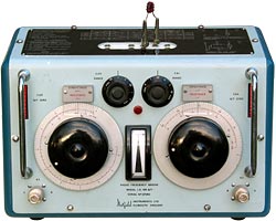
This circuit is based loosely on the 1963-vintage Hatfield Instruments LE300A/1 RF admittance bridge [Handbook ref], for no better reason than that the author happens to own one. The ratio arms of this bridge are formed by two transformers, an isolating transformer with primaries tapped at 1+1 and 10+10 turns, and an auto-transformer that further divides the 1+1 tappings by 10:1. Range switches enable the reference and zeroing elements to be connected to the different ratio-arm taps in order to multiply their influences on the balance condition by 10, 1 or 0.1. In this way, a capacitor of say 250pF can also be used for measurements of 0 to ±25pF and 0 to ±2500pF, and a resistor of say 500Ω can also be used for measurements of 0 to ±50Ω and 0 to ±5KΩ. The influence of the unknown impedance Zx can also be multiplied or divided in the same way, to provide a large selection of measurement ranges (including a remarkable 0 to 2.5pF range); but best accuracy is always obtained when the unknown and the reference components are all set to the same multiplier. DC bias is introduced via a balun transformer with its output in series with the generator, and the reference and zeroing resistors are provided with large series DC-blocking capacitors to ensure that bias current only flows in the device under test. Various trimmer capacitors used for nulling-out stray capacitances have been ommitted for clarity. The transformers can all be wound on high-permeability ferrite beads (e.g., Amidon FT50-43). In the original, the secondary of the ratio-transformer (connected to the generator socket) was 27 turns, and the generator input transformer ratio was 33:11. These transformers are suitable for a generator level of between 100mV and several volts (e.g., a standard lab. signal generator or the transverter output of an HF transceiver), with a short-wave radio receiver as the detector. The author's bridge incidentally came with a built-in crystal-controlled generator and tuned detector operating on 1.591549MHz. This standard measuring frequency is 107 radians/sec, i.e., 2πf=107, a choice that greatly simplifies reactance calculations and corresponds very closely to the low-frequency end of the short-wave spectrum (the medium-wave band ends at 1.6MHz). The manual also states that the bridge can be used up to about 15MHz with an external generator and detector, but in reality, the internal layout is rather expansive and the unit is somewhat inaccurate above about 5MHz.
How to calibrate the universal bridge becomes obvious when the variable resistors are considered as conductances, i.e.:
Gref = 1/Rref
and
Gmin = 1/Rmax
If the reference resistor is rotated to its maximum resistance position, the conductance will not be zero. Also, it is not desirable to have the maximum resistance position at the end-stop, because there may be a resistance step or non-linearity as the wiper moves to the end of the track. The dial is therefore marked zero a little away from the end-stop, and the resistance at the chosen position is measured and designated Rmax. The conductance of the unknown impedance is then given by:
Gx = Gref - Gmin
i.e.,
Gx = (1/Rref) - (1/Rmax)
The quantity Gref-Gmin is marked on the "G" dial, and calibration is established prior to each measurement by setting the "G" dial at zero and adjusting the "Set zero G" resistor until the bridge balances. This calibration step also involves simultaneously setting the "C" dial to zero, and adjusting the "Set zero C" capacitor. For best results, the bridge is re-zeroed after every change of range or frequency.
3-termina measurement and low-impedance adapter
[xx] Hickman's Analog and RF circuits, Ian Hickman. Newnes 1998. ISBN 0 7506 3742 0. p182-
The TRAB, Ian Hickman, EW+WW, Aug. 1994, p670-672.
6-13. Vector and Scalar Addition:
In the AC bridge circuits discussed so far, a voltage detector is used to sample the difference between two points in a network. Because the voltages involved contain phase information, the quantity sampled is a vector sum; and the two voltages are not equal unless they are identical in both magnitude and phase. In some situations however, we wish to ignore the phase information and sample only the magnitudes of the voltages to be compared.
In the context of vectors or phasors, quantities that can be represented by magnitude alone are known as scalars, and the addition or subtraction of such quantities is known as scalar addition. It so happens that the diode detector, by virtue of the smoothing capacitor, removes phase information; which means that scalar voltage addition can be performed provided that the voltages are rectified and smoothed before they are compared. Later on, we will use scalar addition in the design of resistance and conductance bridges that are immune to (i.e., ignore) reactance; but here we will establish the principle by using it to develop a bridge that simply measures impedance magnitude, i.e., |Z|.
6-14. Impedance Magnitude Bridge:
So far we have discussed bridges that represent impedance in its normal R+jX form, and in its reciprocal (admittance) form. There is, of course, another way of representing impedance, which is in terms of magnitude and phase, this being known as the polar form. Bridges that can indicate phase while ignoring magnitude will be discussed in a later section. A bridge that indicates magnitude but ignores phase is shown below:
In this bridge, R0 and ZX share a common current I, and so VX=IZX and V0=IR0. These voltages, of course, contain phase information, and so if we subtract them directly, they only sum to zero when R0 and ZX are identical, i.e., when ZX is real. After rectification and smoothing however, all phase information is lost and we obtain:
V1 = (√2) |VX| - Vf1 = (√2) |I| |ZX| - Vf1
V2 = (√2) |V0| - Vf2 = (√2) |I| R0 - Vf2
where Vf1 and Vf2 are the forward voltage drops of their respective diodes.
Balance occurs when V1=V2; in which case, since both detector loads are identical, the forward voltage drop in D1 will be the same as that in D2 (provided that the diodes are reasonably well matched), and so R0=|ZX|.
Best sensitivity is obtained when the detector input resistance (≈RD/2) is larger than R0 , but the bridge will still balance correctly if it is not because the non-linearities of the two diodes will tend to cancel. For measuring impedance magnitudes of up to about 1KΩ, at frequencies above about 100KHz; RD can be in the range 1 to 10KΩ, and CD about 0.1μF. A suitable choice of meter is 50-0-50μA, with a 100KΩ sensitivity control. A property of this bridge that should be noted incidentally, is that it is not a linear reciprocal network, i.e., there is no definable detector port into which an RF signal can be injected. Notice also that it does not have ratio arms; it works instead by passing the same current through two impedances and comparing the magnitudes of the voltages across them.
One particularly useful feature of the |Z| bridge, and of magnitude bridges in general, is that balance is monitored by means of a centre-zero indicator. This means that that the bridge output contains information regarding the direction in which R0 should be adjusted; which is both convenient for manually operated bridges, and serves as a basis for providing an input to a DC servo amplifier in a self-adjusting system. In order to make the bridge output suitable for driving a servo amplifier however, it is sensible to alter the configuration to that shown below:
In this case, the diode D2 has been reversed. This means that at balance, the two output voltages V1 and V2 are now equal and opposite, and the voltage at the junction of the two equal summing resistors (Rs) is zero. If |ZX| is larger than R0, the input to the amplifier goes positive, and vice versa; and the output of the amplifier can be used to drive a motor, or a voltmeter, or both. In order to avoid loading the detectors, the summing resistors should be at least ten times larger in value than RD, but since the servo amplifier is likely to be based on an operational amplifier with a high input impedance, this is not a problem. In the diagram incidentally, the motor is shown ganged to R0, but it could equally well be ganged to some mechanism that alters the magnitude of ZX, thereby forming part of an automatic impedance matching system.
In the pursuit of automation, the interesting property of an impedance magnitude bridge is that its output is a proper measure of the effect of a transformer in a power transmission system. We noted in [AC Theory, 41], that if an ideal transformer has its secondary winding loaded with an impedance Z, the impedance Z' looking into the primary winding is given by:
| Z' = (Np/Ns)² Z |
6-15. Monitoring Bridges:
In most of the bridges discussed so far, the object of the exercise has been to measure impedance by comparing it against one or more variable reference elements. In antenna matching applications however, it is normal for the bridge ratio to be fixed, and for balance to be achieved by adjusting the load impedance. In this situation, the bridge becomes a monitoring device, i.e., a box of tricks to be inserted in the line between the transmitter and the antenna or matching unit, and it is advantageous to design it in such a way that it absorbs minimal energy from the signals passing through it. Using Christie's circuit (or some AC variant of it) this can be done by reducing the resistance in the current-sampling (reference) arm, and adjusting the ratio arms accordingly, and so our prototype is the arrangement shown below:
The ratio arms (Z1 and Z2) can be resistors, capacitors, or a transformer. Note that the load impedance, being usually an antenna system with a matching network, will probably not have handy controls for independent adjustment of resistance and reactance; but these quantities can nevertheless be manipulated in some way or another. At this point also, we will adopt a consistent notation: Vv for the voltage analog, and Vi for the current analog; and we will start to ignore a redundant property of Christie's bridge, which is that balancing Vv against Vi is the same as balancing the voltage across Z2 against the voltage across the load. If one condition is satisfied, then the other is automatically satisfied, and there is no need to consider them both. For an impedance monitoring bridge, the component values are chosen so that Vv=Vi when the load impedance is equal to the target load impedance, i.e., if the target load impedance is designated R0:
Vv = V Z1 / (Z1 + Z2) = Vi = V Rii / ( Rii + R0 )
which, after rearrangement, gives the balance condition:
| Rii / R0 = Z1 / Z2 |
If the target load impedance is 50Ω, we will presume for now (somewhat unrealistically) that there will be no great difficulty in designing a voltage sampling network (Z1+Z2) that has a reasonably high impedance relative to it. We need to develop a reasonable voltage across the current sampling resistor Rii however, and this implies that there will be a voltage drop in the line resulting from the insertion of the bridge. If we decide that the maximum acceptable voltage drop is (say) 1% (0.09dB), then Rii must be no greater than 0.5Ω, and even at a power level of 100W, |Vi| will only be about 0.7V RMS. This is too low to give good linearity with a simple diode detector, and although we might decide to compensate for the non-linearity, or increase the signal by using amplifiers, we should observe that there is more than enough power available to work a 100μA meter; and we should not be forced to use circuits that need batteries or a mains power supply. The solution is to replace the current sampling element with a step-up transformer; as in the prototype circuit shown below:
The transformer makes it possible to increase |Vi| to a level suitable for a diode detector, or alternatively, it allows the insertion loss (i.e., the power consumed by the current sampling element) to be reduced to a very low level if a low output voltage is acceptable. It also has the significant advantage that it allows the voltage analog Vv and the detector to be referenced to ground; which means that we have the option of dispensing with the diode detector and bringing that end of the transformer to a coax socket. We are then in a position to exploit the fact that the bridge is a linear reciprocal network by injecting a signal of a few tens of milliVolts into the 'detector' port and adjusting the antenna impedance for minimum response at a receiver (i.e., a transceiver switched to receive) connected in place of the generator. In this way, an antenna can be matched ready for transmission without radiating a detectable carrier; the procedure being known as "quiet tuning" [35],[36] or, perhaps more evocatively, "stealth tuning".
Refs:
[35] Simple Quiet Tuning and Matching of Antennas M. J. Underhill G3LHZ, Rad Com, May 1981, p420-422.
The antenna can be matched in receive mode by injecting a small signal into a reverse wave directional coupler in the line to the ATU. The antenna is matched when the level of injected signal heard in the receiver is minimised. The injected signal can be from a noise source, or it can be a comb-spectrum from, say, a crystal calibrator. The injected signal is too weak to interfere with other stations, being undetectable at about 1 wavelength from the antenna.
[36] A Quiet Antenna Tuner, Tony Lymer GM0DHD, QEX May/June 2002, p9-12.
Underhill-Lewis method. QRP single-core version of Sontheimer-Fredrick, performs well from 1.8 - 146MHz.
The bridge now looks very different from Christie's circuit; but the basic principle of operation (the comparison of a voltage analog and a current analog) is the same once the properties of the transformer have been taken into account. Differences to note are that there are now only two voltages, Vv and Vi, to be reconciled (the previously mentioned redundancy has disappeared), and we now have additional parameters; particularly, the transformer turns ratio and the secondary load resistor Ri, which play a part in determining the balance condition. For this reason, Z1 and Z2 are no longer solely responsible for determining the ratio between the current and voltage samples, and should no longer be described as ratio arms. Instead, Z1 and Z2 form a voltage sampling network, and the transformer and its secondary load form a current sampling network. A transformer in this application is called a current transformer, and as we shall see in the next section, the resistor Ri that shunts the secondary is essential for the production of an output voltage proportional to and approximately in phase with the current.
© D W Knight 2007.
David Knight asserts the right to be recognised as the author of this work.
Further Work
Topics that perhaps ought to be added:
A. Table of common bridge types + a few more obscure ones
B. Obtaining information from out-of balance bridges.
C. Complex Z measurement using only scalar voltage measurements.
Strandlund, QST, June 1965, p24-28.
Gruchalla, CQ, Fall 1998, p33-43
The MFJ 269 antenna analyser (for example), uses scalar addition of voltages from a simple symmetric resistor ratio-arm bridge.
Despite the alarming lack of quantitative information in the manual on the subject of instrumental accuracy; the author's MFJ-269 gives good inductance measurements. Readings in the region of 10 μH at the lowest working frequency (1.7 MHz) agree within 2% with measurements made using a Hatfield LE-300/A1 at 1.5915 MHz (error ±0.5%).
The facility for capacitance measurement appears somewhat crude by comparison: readout is to the nearest pF and error is about 10% in the region of 100 pF; but this limitation can be worked around with the aid of a calculator. The trick is to use the displayed reactances and subtract an offset for the jig capacitance, all of which can be done using readings from the instrument itself. It is possible in this way to measure small capacitances to about 1 decimal place in pF, making the MFJ-269 useful in the lab. as well as when fettling antennas.
| |
|
|
|
|