|
|
|
|
|
|
2. Components and Materials: Part 1.
Contents:
|
1. Resistance, resistors and conductors. 2. Skin effect. 2a. AC resistance of thick wires. 3. Traditional approximations for Rac. |
3a. AC Resistance factor. 4. Conductor Perimiter. 5. Proximity effect. . |
| The analytical separability of resistance and reactance that underpins AC circuit analysis can lead to the impression that, were it not for the limitations of the materials at our disposal, it might be possible to create perfect passive components. This, as it transpires, is not the case; for reasons that are embedded in electromagnetic theory, and that can ultimately be traced to the principle of causality [1]. It can be shown that, if the relationship between resistance and reactance is assumed to be arbitrary, then it it is implied that there are networks that can see into the future (i.e., systems that give an output before receiving an input). It is not possible to build such circuits, and the consequence is that there are constraints on the impedances that can be exhibited by any given device. Thus the bad news is that there are no ideal resistors, capacitors, and inductors; the best we can do is to optimise a component for one of the three attributes and try to minimise the others. The good news however, is that we can still analyse most circuits as though they are made up of hypothetical pure resistances and reactances; i.e., it is legitimate to draw equivalent circuits for our imperfect components and so produce theoretical models that describe practical networks to a high degree of accuracy. In some instances, a simple analysis based on the idea that electronic components are ideal is sufficient; but such an approach is often inadequate at radio frequencies. It is therefore important that we develop at least a qualitative, and preferably a quantitative, understanding of the properties of practical electrical components (and that includes wires, circuit-board tracks, and insulators); and so we return to basics and look once again at the subjects of resistance, capacitance, and inductance. |
|
1. Resistance: Resistors and Conductors: Forgive us for stating the obvious; but resistance is an attribute of objects that conduct electricity, whereas a resistor is an electrically conductive device designed to exhibit a particular value of resistance over a reasonable range of temperatures, voltages, and frequencies. Thus 'resistor' and 'resistance' are quite different concepts, and it is important to be sure of the distinction. Resistance is a dynamic manifestation of the ability to consume power or perform work (both being equivalent from a circuit analysis point-of-view), and there can be no resistance when there is nothing to resist. Consequently, in the absence of an applied voltage, resistance exists only notionally as a predictor of the corresponding current when a particular voltage is applied. If a voltage is applied to a resistance, an electric field must exist in the vicinity of that resistance (electric field-strength is measured in volts per metre). If an electric field exists, energy must be stored in that field or as a result of the forces produced by that field. Therefore resistance cannot exist independently of capacitance. If a voltage is applied to a resistance, a current flows, i.e., a magnetic field is formed, and energy is stored in that field or as a result of the forces due to that field. Therefore resistance cannot exist independently of inductance. Since resistance cannot exist independently of inductance and capacitance, the impedance presented by any resistor or conductor carrying an electrical current will always vary with frequency. It transpires that the real part of that impedance, the effective resistance, will also vary with frequency; for reasons associated with the way in which resistance and reactance interact. If a very pure (i.e., frequency-independent) resistance is required (e.g., for a dummy-load resistor), about the best we can do is construct a low-value resistor as part of a transmission-line; i.e., place it in a metal tube with dimensions calculated to give a particular characteristic impedance, like a coaxial cable. A transmission-line is a device in which the distributed inductance of the conductors is balanced by the distributed capacitance between the conductors at all frequencies, provided that the line has no losses and is terminated by a particular value of resistance. Unfortunately, transmission-lines do have losses, and there will be some difficulty in determining where the transmission line ends and the resistor begins; which means that there will always be a small residual reactance. Thus, whatever we do, pure resistance always eludes us, and although the frequency dependence can be minimised, it can never quite be made to go away. |
|
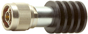
50 Ω, 3 W coaxial resistor mounted on an
N-type connector (TME model CT-03. Overall length 63 mm). Provides an almost purely resistive termination at frequencies up to 1 GHz. |
 |
|
In any electrical system, energy is transported by the electromagnetic
field. Hence the electric 'current' used in calculating power
is associated with the magnetomotive force, and is identical
to the magnetomotive force in the event that each loop of magnetic
flux encirles the current only once (i.e., presuming that the
conductors are not coiled). The magnetic field however sets charges
(e.g.., free electrons in wires) in motion, and so there is a
current (sometimes called convection current) within conductors,
and this current is proportional to the strength of the magnetic
field. The fields due to the conduction current and the incident
electromagnetic energy interact (i.e., are superposed) in such
a way as to cause energy to follow the outside surfaces of conductors.
Thus electrical energy is guided by wires, but remains largely
external to them. Because electrons undergo collisions with the atoms of the materials in which they move, the conduction process is not perfectly efficient. The energy transferred by collisions is lost from the field and converted into heat. Thus we pay a price for the facility to guide energy from place to place, in that conductors offer resistance to the flow of current. The resistive loss is proportional to the current density, i.e., to the conduction current per unit area at some point in a plane perpendicular to the direction of flow. Hence losses can be reduced by increasing the available area; but (as we shall see in the next section) it turns out that, except at very low frequencies, increasing the effective area for conduction is not the same as increasing the cross-sectional area of the conductor. |
|
2. Skin Effect: The resistance of ordinary conductors, although often considered to be negligible, increases drastically with frequency. This is due to a phenomenon known as the skin effect; which arises because the conduction current at the surface of a conductor prevents the associated magnetic field from penetrating into the body of the conductor. Since a current always has a magnetic field associated with it; the result is that the current becomes more and more concentrated at the surface as the frequency is increased [2]-[5]. From a radio engineering point of view, the major consequence of the skin effect is that the high-frequency resistance of wires and other low-resistance conductors is much greater than the DC resistance. This phenomenon is the principal cause of energy loss in transmission lines, antenna wires and coils, and must therefore be taken into account when maximising the efficiency of RF power-transmission equipment. The variation of resistance with frequency for a conductor is a function of its conductivity and its magnetic permeability, both of which will be defined in the discussion to follow. |
For a resistor or conductor of uniform composition carrying a
direct current; resistance can be defined in terms of a bulk
property of the conductive material called its volume resistivity,
or just plain 'resistivity' [6].
Resistivity is usually given the symbol 'ρ' (Greek
lower-case letter 'rho'). The DC resistance of a uniform conductor
is proportional to its length, and inversely proportional to
its cross-sectional area, and ρ is the constant of
proportionality; i.e.:
|
 |
|
If length is measured in metres, and area is measured in metres-squared,
then resistivity must be measured in Ohm-metres (Ωm) in
order for the right-hand side of this equation to have overall
dimensions of Ohms (Ohm metres × metres / metres²
= Ohms). In some reference books however, resistivities are given
in Ωcm. To convert a quantity in Ωcm to Ωm,
divide it by 100. The table below shows the resistivities of some common materials in nano-Ohm-metres, i.e., Ωm×10-9. |
| Material | Notes |
@ 20°C / nΩm |
/ per K |
expansion / per K |
| Aluminium, Al | 28.24 | 0.0039 | ||
| Brass | Cu 56-61%, Zn, Pb 1.5-3.5%. | ~70 | 0.002 | |
| Constantan (Eureka) | Cu 60%, Ni 40%. | 490 | 0.000008 | 14.9 ×10⁻⁶ |
| Copper, Cu | Annealed | 17.241(1) | 0.00393 | 16.5 ×10⁻⁶ |
| Hard-drawn | 17.71 | 0.00382 | ||
| Gold, Au | Pure | 24.4 | 0.0034 | |
| Iron, Fe | Fe 98.5 - 99.98 %, remainder C | 100 | 0.005 | |
| Kovar(2), Rodar, Fernico 1. | Fe 53%, Ni 29%, Co 17% | 490 | 5 ×10⁻⁶ | |
| Lead, Pb | 220 | 0.0039 | ||
| Manganin | Cu 84%, Mn 12%, Ni 4%. | 440 | 0.00001 | |
| Mercury, Hg | (3) |
957.83 (940.734 @ 0°C) |
0.00089 | |
| Nichrome | Ni 80%, Cr 20%. | 1000 | 0.0004 | |
| Nickel, Ni | 78 | 0.006 | 13.4 ×10⁻⁶ | |
| Phosphor bronze | Cu, Sn 9-13%, P 0.3-1%. | 78 | 0.0018 | |
| Platinum, Pt | 105 | 0.003 | 8.8 ×10⁻⁶ | |
| Silver, Ag | 15.87 | 0.0038 | 18.9 ×10⁻⁶ | |
| Solder, 60/40 | Sn 59.5-61.5%, remainder Pb | 149.9 (25°C) | ||
| Tin, Sn | 115 | 0.0042 | ||
| Tungsten, W | (2) | 52.8 | 4.5 ×10⁻⁶ | |
| Zinc, Zn | 58 | 0.0037 |
|
(Sources: CRC Handbook [7],
see also Kaye & Laby online [8]
& Wikipedia. Solder resistivity from manufacturer's data
sheet). (1) International Annealed Copper Standard [51] (2) Used for glass-to-metal seals in borosilicate glass. (3) The international standard Ohm was once defined as the resistance of a column of pure mercury with a cross-sectional area of 1 mm² (i.e., 10-6 m²) and a length 1.063 m, maintained at 0°C. Using ρl/A=1, this gives ρ=10-6/1.063 = 940.734 nΩm @ 0°C. The modern definition of the Ohm is based on the von Klitzing resistance RvK, determined from the Quantum Hall Effect [45]. RvK = 25812.8056 Ω. |
The table does not show all of the possible materials that can
be used to make conductors at normal temperatures, but it does
show the best ones. These are, in order of increasing resistivity;
Silver, Copper, Gold, and Aluminium. Notice also, that alloying
increases resistivity, so that pure metals are the best conductors
(although not necessarily best at resisting atmospheric attack).
The alloys constantan and manganin are used in the manufacture
of wirewound resistors and potentiometers, and are favoured for
their high resistivities and low temperature coefficients (ref
[8], section 1.8.2). Nichrome
is the resistance-wire alloy used in electric fires and heating
elements, and is favoured for its ability to resist oxidation
at temperatures up to 1000°C (i.e. when glowing red hot).
Observe that the resistivities listed in the table are mostly
given at a temperature of 20°C. If we call this reference
temperature T0, and the resistivity at
this temperature ρ0, then the
resistivity at some other temperature T can be calculated using
the temperature coefficient α (alpha) as follows:
ρ = 17.241 × (1 - 5×0.00393) = 17.241 × 0.98035 = 16.90 nΩm. Evidently, copper would not be much good for making resistors even if it had a higher resistivity, because its resistance changes by 2% for a mere 5° change in temperature. In general, resistivities calculated using temperature coefficients are less accurate than the resistivity at the measurement temperature T0; and resistivity data should always be sought for a temperature close to the required temperature (see ref [8], section 1.8.1). Note that the temperature coefficient is always positive for true conductors, but is negative for semiconductors; i.e., as the temperature is increased, conductors increase in resistance, and semiconductors reduce in resistance. >>>> Insert passage on inferred absolute zero method. At high frequencies, conduction current is confined to a shallow region at the surface, this being the depth to which electromagnetic energy of a particular frequency can penetrate. If we assign the symbol δi (Greek lower case "delta") to this penetration depth or "skin depth", it is given by the expression:
σ (Greek lower-case "sigma") is the conductivity of the material, and is simply the reciprocal of the resistivity, i.e.,:
μ (Greek lower-case "mu") is the magnetic permeability of the material [6], and is defined as:
χ(cgs)=(μr-1)/4π. The dimensionless susceptibility in the cgs system must therefore be multiplied by 4π to make it consistent with the SI definition. AC measurement of magnetic susceptibility is also possible and is used for the characterisation of non-conducting materials and superconductors [50]. Materials can be classified into three principal types according to their magnetic susceptibilities; these are: diamagnetic, paramagnetic, and ferromagnetic. Diamagnetic materials are less permeable than free space, and therefore experience a small repulsive force when introduced to the field between the poles of a magnet. Typical diamagnetic susceptibilities are in the order of -10-5; and so diamagnetism decreases the permeability of a material in comparison to free space by about 0.001%, and can therefore be ignored when estimating RF resistance. Paramagnetic materials are more permeable than free space and so are attracted into magnetic fields; but the effect is once again small, typical paramagnetic susceptibility being in the order of +10-3, i.e., paramagnetism increases the permeability by about 0.1% in comparison to free space and can also be ignored. Ferromagnetism however, is a special case of paramagnetism, it being associated with extremely large magnetic susceptibilities; more than one million for some special magnetic alloys. The relative permeability of ferromagnetic materials varies with the magnetic field strength, and such materials will always show some residual magnetisation when the magnetising force is removed. Ferromagnetism also disappears above a certain temperature, known as the Curie point, which depends on the material (the Curie point for iron is 770°C). One obvious test for ferromagnetism is to see if the material can be picked-up with a permanent magnet. The table below shows the susceptibilities and permeabilities of the common wire-making and wire-plating materials . The permeabilities of the ferromagnetic materials are necessarily approximate, the appropriate figure for the present purpose being the initial permeability, i.e., the permeability associated with low values of magnetic field strength. |
| Material | Susceptibility χ | @ temp | Relative permeability μr=(1+χ) |
| Aluminium, Al | +2.21 × 10⁻⁵ | 1.00002212 | |
| Copper, Cu | -9.56 × 10⁻⁶ | 23°C | 0.99999044 |
| Gold, Au | -3.66 × 10⁻⁵ | 23°C | 0.99996337 |
| Iron, Fe (0.1% C) | ferromagnetic | 200 (initial, 20 gauss) | |
| Lead, Pb | -1.70 × 10⁻⁵ | 16°C | 0.99998299 |
| Nickel, Ni | ferromagnetic | 250 (initial) | |
| Platinum, Pt | +2.62 × 10⁻⁴ | 1.0002617 | |
| Silver, Ag | -2.63 × 10⁻⁵ | 23°C | 0.9999738 |
| Tin, Sn (white) | +2.40 × 10⁻⁶ | 1.0000024 | |
| Tin, Sn (grey)* | -2.85 × 10⁻⁵ | 7°C | 0.9999715 |
| Zinc, Zn | -1.56 × 10⁻⁵ | 0.9999844 |
|
(sources: Refs [7] and [8]) *Grey tin, the preferred crystalline form below 13°C, is also known as 'tin pest' (a degenerative disease of electronic equipment built using some types of unleaded solder). |
With resistivity and permeability data thus obtained from standard
reference books, we are in a position to calculate the skin-depth
and resistance per unit length at various frequencies for a selection
of representative conductors. Using equation (2.2)
given earlier, the skin-depth can be written:
|
Conduction layer thickness in microns:
|
Material |
|
|
|
|
|
|
|
σ / MS/m |
|
|
|
|
|
|
|
μr |
|
|
|
|
|
|
|
r e q _ M H z |
|
|
|
|
|
|
|
|
|
|
|
|
|
|
|
|
|
|
|
|
|
|
|
|
|
|
|
|
|
|
|
|
|
|
|
|
|
|
|
|
|
|
|
|
|
|
|
|
|
|
|
|
|
|
|
|
|
|
|
|
|
|
|
|
|
|
|
|
|
|
|
|
|
|
|
|
|
|
|
|
|
|
|
|
|
|
|
|
|
|
|
|
|
|
|
|
|
|
|
|
|
|
|
|
|
|
|
|
|
|
| The surprise is perhaps that the current-carrying layer is extremely thin even at low radio frequencies; the skin-depth in copper (for example) being only 48 μm (0.048 mm) at 1.9 MHz. Notice also that the ferromagnetism of iron has a devastating effect on the skin-depth, even though iron is a material of relatively low conductivity. A recent recommendation in a British Amateur-Radio magazine, that plastic-covered iron wire sold in Garden Centres can be used to make aerials, does not seem so sensible in light of these calculations. It will seem even less sensible when we estimate the actual resistance per unit length of some typical wires. |
|
2-2a. AC resistance of thick wires. Using equation (2.1) given earlier, the resistance per unit length of a conductor can be written: R / l = ρ / Aeff where Aeff is the effective conductor area, which is a function of the skin-depth δi and the shape of the conductor cross section. |
|
The diagram on the right represents the cross section of a cylindrical
wire of radius r (and diameter 2r). The full area A of the conductor
is: A = π r² but the effective area for RF conduction is: Aeff = πr² - π(r - δi)² (i.e., the area of the outer circle minus the area of the inner circle) Expanding the term in brackets gives: Aeff = π (r² -r² +2rδi -δi²) i.e.,
|
 |
Strictly, the equation above is valid provided that r is greater
than δi (i.e., r>δi), but obviously, we want to use it in conjunction
with skin-depth data calculated using equation (2.2),
and equation (2.2) is a solution
of Maxwell's equations for a plane (flat) conductor. Therefore
we specify that r should be much greater than δi (r>>δi),
thereby ensuring that the curvature of the conductor is small
in comparison to the skin depth, so that the assumption of planarity
(flatness) remains valid. The resistance per unit length of a
conductor at radio frequencies (combining equations 2.1 and 2.4)
is then:
|
| The table below shows the resistance per metre of 1.5mm diameter wires made from various common metals calculated using equation (2.5): |
Resistance (in Ohms) of a 1 m length of 1.5 mm diameter wire.
|
Material |
|
|
|
|
|
|
|
ρ / nΩm |
|
|
|
|
|
|
|
r e q / M H z |
|
|
|
|
|
|
|
|
|
|
|
|
|
|
|
|
|
|
|
|
|
|
|
|
|
|
|
|
|
|
|
|
|
|
|
|
|
|
|
|
|
|
|
|
|
|
|
|
|
|
|
|
|
|
|
|
|
|
|
|
|
|
|
|
|
|
|
|
|
|
|
|
|
|
|
|
|
|
|
|
|
|
|
|
|
|
|
|
|
|
|
|
|
|
|
|
|
|
|
|
|
|
|
|
|
|
|
|
|
|
|
We do not of course, normally encounter wires made of solid silver,
zinc, or tin. These are instead the common plating materials.
Typically, a silver-plated copper wire will have a plating thickness
of 1-10 μm, a tin-plated copper wire will have a plating thickness
of about 0.8-3 μm, and a heavy-zinc plated (hot-dip galvanised)
iron fencing-wire about 50-125 μm [data culled from various
wire manufacturer's websites]. Once the skin-depth becomes substantially
less than the plating thickness, practically all of the radio-frequency
current flows in the plating, and the resistivity of the base-wire
becomes irrelevant [9]. Notice
also that for radio-frequency purposes, a tubular conductor is
just as good as a solid wire, and may offer a considerable saving
in weight and cost when a large diameter is required. The data in the table above indicate that silver-plated copper wire or tubing is the best commonly available conductor for radio applications, with plain copper (bare or enamel coated) coming a close second. Tin-plated copper (ordinary hook-up wire) is somewhat inferior, and although the current will tend to penetrate into the underlying metal even at UHF, considerable current density will still occur in the high-resistivity outer layer. An interesting corollary here is that solder (60/40 tin-lead alloy) has a higher resistivity than plain white-tin, and so when soldered joints are made, care should be taken to minimise the spread of the solder. This is not a serious issue when making wire connections, but it does mean that the RF signal tracks of printed circuit boards should be left as plain copper as far as possible, a layer of protective lacquer being preferable to solder-coating. Having praised silver however, we should state that there is some controversy over the matter of whether or not the silver plating of copper conductors is worthwhile [2][12], especially since the reduction in surface resistivity is only about 7.8%. The issue here is that silver plating definitely reduces RF resistance initially; but if the silver is allowed to tarnish, the RF resistance will eventually exceed that which can be achieved using plain-copper that has been subjected to the same environmental conditions. We can understand what is happening here by noting that both silver and copper will grow a surface layer on exposure to the atmosphere. In the case of copper this will be composed of copper oxides (and will include a mixture of copper hydroxide and carbonate if the wire goes green), whereas in the case of silver; the surface layer is composed mainly of silver sulphide. If the tarnish layer is moderately conductive, either throughout, or in the partially-formed boundary layer between it and the metal, some of the conduction current will flow in the tarnish layer, and this process will be lossy. Consequently, we can deduce that if the Q of silver resonators (for example) degrades faster than the Q of copper resonators (which it does), then either silver sulphide is a much poorer insulator than copper oxide, or the partially-conductive boundary between the metal and the non-conductive tarnish coat is thicker in silver than it is in copper. The former appears to be the case, since the resistivity of AgS is around 1.5 - 2.0 Ωm, whereas for CuO it is 6 kΩm and for Cu2O it is 10 - 50 Ωm [13] (Ag2S is light-sensitive and so cannot be expected to persist). The conclusion in any case is that silver plating is only worthwhile if the silver is sealed away from environmental contamination and sources of sulphur (such as vulcanised rubber). We should note also, that enamel-coated copper will not tarnish at all, and so should maintain its initial performance indefinitely; and the increase in losses for not using silver can often be offset simply by increasing the wire diameter. For truly dire performance however, soft-iron garden-wire is in a class of its own (although galvanised-iron fencing wire is not too bad, except that it will eventually rust). A 10 m long transmission-line made from plain iron wire (1.5 mm diameter) would have a loss-resistance in the region of 140 Ω at 14 MHz. The only saving grace, is that the author of the recommendation that it can be used to make antennas will be hampered in passing-on his ideas via radio. Condemnation aside however, this does raise an interesting issue; which is that VHF mobile radio installations often use stainless-steel whip antennas, and the question arises as to whether or not this is a good idea. The author owns a 2m-band mobile antenna, and the whip is made from a 2.5 mm diameter stainless-steel rod that is distinctly ferromagnetic. Most stainless-steels are austenitic, i.e., they contain iron in its non-magnetic form (austenite), and so the rod is probably made from type 301 alloy (Fe 74.6%, Cr 17.6%, Ni 7.8%) (ref [8], p146). This has a relative permeability of 14.8 in its magnetic (ferritic) form, and a resistivity of 68 nΩm (σ=14.7 MS/m). The skin depth for this material at 145 MHz (using equation 2.3) is: δi = 503.292121 / √( 145 × 106× 14.8 × 14.7 × 106 ) = 2.83 μm The antenna is a so-called 5/8-wavelength vertical. A proper description is that it is a shortened 3/4-wavelength (0.75λ) ground-plane antenna. The input impedance of a vertical antenna changes cyclically as the length is increased, crossing the resistance axis (i.e., X→0) with alternating low and high input resistance every time the length reaches a whole number of electrical quarter-wavelengths (electrical length is always slightly longer than physical length, due to a reduction in the apparent speed of light for waves travelling in the vicinity of conductors). A perfect vertical antenna mounted on a perfect ground plane has an input resistance of about 36.6 Ω when its electrical length is 0.25λ, and about 45 Ω when its electrical length is 0.75λ (the painted mild-steel roof of a car is not a perfect ground plane, but it is a lot better than soil). The effect of shortening a 0.75λ vertical antenna slightly is to increase its input resistance and make the input impedance capacitively reactive. To make the antenna suitable for connection to a 50 Ω coaxial cable therefore, it is shortened slightly to raise its input resistance, and a loading coil is added to cancel the resulting reactance. The length of the antenna is thus chosen so that the radiation resistance, plus the loss resistances of the antenna hardware and the loading coil, add up to 50 Ω. The stainless-steel rod part of the author's antenna is 1.17 m long (this is not the whole of the antenna length, because some of it is made up by the loading coil and mounting hardware). The resistance at 145 MHz of this length of 2.5 mm diameter SS301 rod is: R = ρ l / [π (2rδi - δi²) ] = 68×10-9 × 1.17 / (22.201×10⁻⁹) = 3.58 Ω Not all of this resistance appears in the antenna input impedance however, because the current-distribution in the whip is not uniform (the current goes to zero at the top). In fact, on the assumption that the current distribution is sinusoidal, the contribution is about half the resistance of the rod, i.e., about 1.8Ω. Consequently, the resistance of the rod consumes about 1.8/50, i.e., about 3.6% of the transmitter power. This is a very small loss in signal-strength terms: 20log[48.2/50] = -0.32 dB and so, despite the unprepossessing resistivity of the rod material, the choice is harmless in this case. Indeed, the resistance of the rod is beneficial, because it provides the antenna with a small amount of resistive loading (in addition to that due to the roof of the car), and so reduces the Q and helps to make the antenna usable without adjustment over a band of several MHz. |
|
2-3. Traditional approximations for AC resistance: The RF resistance of a cylindrical conductor in the thick conductor approximation is given by a slight rearrangement of equation (2.5):
R = ρ l / (π2r δi ) r >> δi or, using the wire diameter instead of the radius: R = ρ l / (πd δi ) d >> δi Now using equation (2.3) given earlier, we can eliminate δi, i.e.: R = ρ l [√( π f μ0 μr σ )] / (π d ) f >>0 or, using σ = 1/ρ : R = ρ l [√( π f μ0 μr )] / (π d [√ρ]) Dividing a number by its square-root is the same as taking the square-root (i.e., a number may be considered to be the square of its own square-root), and so ρ/√ρ=√ρ and (√π)/π=1/(√π), hence:
This expression can be further reduced for specific materials, as in the table below: |
Table 3#1: Approximate RF resistance of cylindrical conductors:
| Conductor |
ρ / nΩm (at 20°C) |
RF resistance / Ω (f is in Hz. l and d must have the same units) |
| Silver | 15.9 | R = 7.975×10⁻⁸ (√f ) l / d |
| Copper, annealed (soft). | 17.241 | R = 8.304×10⁻⁸ (√f ) l / d |
| Copper, hard-drawn | 17.71 | R = 8.417×10⁻⁸ (√f ) l / d |
| Aluminium | 28.24 | R = 10.628×10⁻⁸ (√f ) l / d |
|
|
|
2-3a. AC-Resistance factor: It is often useful to express the AC resistance of a wire as a factor of the DC resistance, i.e.: Rac = Rdc Ξ Where Ξ (Greek capital Xi) is the factor by which the DC resistance is increased as a result of the skin effect. From equation (2.1) the DC resistance is: Rdc = ρ l / A and the AC resistance is: Rac = ρ l / Aeff Hence: ρl / Aeff = Ξ ρl / A i.e., Ξ = A / Aeff where A=πr² for a solid cylinder and, from equation (2.4): Aeff = π (2rδi - δi²) Hence the skin-effect factor (in the high-frequency / thick-conductor approximation) is:
For best accuracy, Ξ should be evaluated in full; but in old textbooks and papers the δi² term is dropped for reasons of computational expediency. Hence: Ξ = r / (2δi) The diameter of the wire is generally preferable to the radius, since diameter is the quantity actually measured, hence: Ξ = d / (4δi) Substituting for δi gives:: Ξ = (d / 4) √( π f μ0 μr / ρ ) and if non-ferromagnetic material is assumed, μr=1. We can also insert the value μ0=4π×10-7H/m to obtain: Ξ = (d / 4) √( 4×10⁻⁷ π² f / ρ ) which, after factoring 4π² from the square-root bracket and rearranging, gives:
Ξ = 3.78 (d/[mm])×10-3 √ (106×f/[MHz]) we can see that the the 106 inside the square-root bracket cancels the 10-3 outside the square-root bracket, and so the formula is good for MHz and millimetres, i.e.: Ξ = 3.78 (d/[mm]) √(f/[MHz]) Hence for an isolated 1mm diameter copper wire operating at 1 MHz, equation (3.4) tells us that the AC resistance is roughly 3.8 times the DC resistance. |
|
2-4. Conductor Perimeter: For direct currents, the resistance of a conductor is inversely proportional to its cross sectional area; but at high frequencies, due to the skin effect, its resistance is inversely proportional to its perimeter. The perimeter of a circle is, of course, the circumference (which is equal to π×d), and so the RF resistance of a cylindrical conductor decreases as the diameter is increased. It should be noted however, that a circle is the shape that gives the shortest perimeter for a given area; and so the RF resistance of conductors can be reduced by deviating from a circular cross-section. This observation results in the use of flat copper (or silver-plated copper) strip for conductors and coils in high-power high-frequency RF applications [3], and in the use of bunch-wire and litzendraht (woven-wire) at lower frequencies (10 kHz - 3 MHz). |
|
|
Bunch-wire |
| Bunch-wire is made simply by taking several strands of insulated (usually enamelled) wire and twisting them together. The wires are kept electrically separate, and are not stripped of insulation and soldered together until they reach their terminations. The idealised cross-section for a bunch of seven wires is shown in the illustration right. Notice that the overall diameter D in this case is three times the diameter of of the wires used, i.e., the wire diameter is D/3. The circumference of each wire is therefore πD/3, and since there are seven strands, the total perimeter is 7πD/3 (assuming that the insulation is very thin). Thus, by using seven strands we increase the perimeter by a factor of very nearly 7/3 (2.33) compared to a solid cylindrical wire of the same overall diameter. |
 |
|
From the above argument, we might
be tempted to assume that a seven-strand bunch will have an RF
resistance that is 3/7 of that of a comparable single wire, but
unfortunately, this is not the case. Such a topology does reduce
the effective resistance significantly at very low radio-frequencies,
but its usefulness fades as the frequency is increased. The reason
can be seen by first considering the points at which the wires
lie in contact with each-other. Here, for a particular wire,
the field associated with the current in the adjacent wire will
be strong; and at some fairly low frequency, by the same process
as that which gives rise to the skin-effect, these regions will
cease to carry significant current. Once current has been repelled
from these regions, the wire surfaces facing into the six voids
inside the bundle will be screened from the outside world, and
current will only flow on the outward-facing surfaces. At this
point, the central conductor carries virtually no current and
serves no purpose except to maintain the shape of the bundle.
As the frequency is increased further, current will not even
venture into the valleys between the conductors, at which point
the RF resistance will be much the same as that obtained by using
a single wire of the same overall diameter. It is for this reason
that, although bunch-wire is used for coils and interconnections
in switched-mode power converters (tens of kHz), it is not much
used in HF radio applications. Litzendraht or "Litz wire" gives an improvement in high-frequency performance in comparison to bunch-wire because it is woven in such a way that, in a given length, every conductor has an equal chance of appearing in the outside layer of the bundle (i.e., it is braided or plaited). In this way, no conductor is completely buried, and every conductor is forced to carry current. The use of litz wire is generally beneficial between about 50 kHz and 3 MHz [14][15], but offers only marginal advantage at the higher end of this range (i.e., on the 160m band). Litz wire, incidentally, is also sometimes used in audio systems. It serves no useful electrical purpose at audio frequencies, because the skin depth is greater than the radius of all reasonably-sized wires, and its bulk (DC) conductivity is less than that of solid or multi-strand wire of the same overall diameter. It is much more expensive than ordinary wire however, and in Hi-Fi circles that alone appears to be sufficient reason for using it. |
|
|
|
2-5. Proximity effect: |
© D W Knight 2008, 2014
David Knight asserts the right to be recognised as the author of this work.
|
|
|
|
|